
Optimal Control of a Variable-Mass Thrust-Vectoring Lander
Spring 2026 MAE 270C
Nathan Ge
Abstract
This project studies the optimal guidance and control of a planar variable-mass rocket/lander with translational and rotational dynamics, bounded controls, nonlinear coupling, free-final-time optimal control, endpoint manifold constraints, and trajectory tracking. It combines Pontryagin’s Maximum Principle (PMP), controllability analysis, Linear Quadratic Regulation (LQR), minimum-time optimal control, nonlinear indirect optimal control, and numerical two-point boundary value problem (TPBVP) solvers. The work is inspired by powered-descent guidance and reusable rocket landing systems studied in modern aerospace optimal control literature. All theoretical derivations are based on PMP; numerical implementations use indirect shooting, collocation, and hybrid approaches, with every optimality condition derived from PMP.
The project is structured in four parts, each of which perturbs a single ingredient of one shared optimal control problem — the cost, the endpoint conditions, the final time, or the plant. Section II derives that shared skeleton once; Sections IV–VII state only what each part changes.
I. Problem Formulation
The lander is modeled as a planar rigid body with variable mass, thrust-vectoring, and torque authority. The state and control vectors are
\[x = \begin{bmatrix} p_x & p_z & v_x & v_z & \theta & \omega & m \end{bmatrix}^{\top}, \qquad u = \begin{bmatrix} \delta T & \tau \end{bmatrix}^{\top}\]| Symbol | Description |
|---|---|
| $p_x,\ p_z$ | Horizontal and vertical position |
| $v_x,\ v_z$ | Horizontal and vertical velocity |
| $\theta$ | Vehicle pitch angle |
| $\omega$ | Angular velocity (pitch rate) |
| $m$ | Instantaneous vehicle mass |
| $T$ | Commanded thrust magnitude |
| $\tau$ | Commanded control torque |
The nonlinear equations of motion $\dot{x} = f(x,u)$ are defined by kinematics, gravity, thrust resolution, and mass depletion:
\[\dot{x} = \begin{bmatrix} v_x \\ v_z \\ -\dfrac{T}{m}\sin\theta \\ \dfrac{T}{m}\cos\theta - g \\ \omega \\ \dfrac{\tau}{I} \\ -\alpha T \end{bmatrix}\]where $\alpha = 1/(I_{sp}g_0)$ is the propellant consumption rate. Throughout Parts I, II and IV the control is the thrust increment about the hover trim, $\delta T = T - m_0 g$, so that $T = m_0 g + \delta T$.
Constraints
| Constraint | Description |
|---|---|
| $T \in [T_{\min}, T_{\max}]$ | Actuator bounds on thrust magnitude |
| $\tau \in [\tau_{\min}, \tau_{\max}]$ | Actuator bounds on control torque |
| $p_z(t) \geq 0$ | Hard deck limit preventing subsurface flight |
| $m(t) \geq m_{\text{dry}}$ | Minimum mass limit (dry mass) |
Parameters
| Symbol | Value | Description |
|---|---|---|
| $g$ | 9.81 m/s² | Gravitational acceleration |
| $I$ | 10 kg·m² | Vehicle moment of inertia |
| $m_0$ | 20 kg | Initial vehicle mass |
| $\alpha$ | 0.005 kg/(N·s) | Propellant consumption rate |
| $T_{\min}$ | 0 N | Minimum thrust limit |
| $T_{\max}$ | 300 N | Maximum thrust limit |
| $\tau_{\min}$ | −30 N·m | Minimum torque limit |
| $\tau_{\max}$ | 30 N·m | Maximum torque limit |
II. The PMP Skeleton
Every part of this project is an instance of the same necessary-condition machinery. Deriving it once makes the four parts readable as variations rather than four separate problems.
Base Derivation
Given a running cost $L(x,u)$, a terminal cost $\varphi(x(t_f))$, and dynamics $\dot{x} = f(x,u)$, the Hamiltonian adjoins the dynamics to the cost through the costate $p$:
\[H(x,u,p) = L(x,u) + p^{\top} f(x,u)\]PMP then supplies three conditions. The adjoint (costate) equation propagates $p$ backward:
\[\dot{p} = -\frac{\partial H}{\partial x}\]The stationarity condition selects the control that minimizes $H$ pointwise over the admissible set:
\[\frac{\partial H}{\partial u} = 0\]And the transversality condition closes the system at the terminal time:
\[p(t_f) = \left.\frac{\partial \varphi}{\partial x}\right|_{t=t_f}\]For the quadratic cost $L = x^{\top}Qx + u^{\top}Ru$ on the linearized plant $\dot{x} = Ax + Bu$, these evaluate to
\[H = x^{\top}Qx + u^{\top}Ru + p^{\top}(Ax+Bu), \qquad \dot{p} = -2Qx - A^{\top}p, \qquad u^{*} = -\tfrac{1}{2}R^{-1}B^{\top}p\]The Riccati Substitution
For the linear-quadratic parts the TPBVP admits a closed-form reduction. Assume the costate is linear in the state, $p(t) = P(t)x(t)$, with $P$ an unknown time-varying symmetric matrix. Differentiating,
\[\dot{p} = \dot{P}x + P\dot{x}\]Substituting the adjoint equation on the left, the dynamics on the right, and $u^{*} = -\tfrac{1}{2}R^{-1}B^{\top}Px$:
\[-2Qx - A^{\top}Px = \dot{P}x + P\left(Ax - \tfrac{1}{2}BR^{-1}B^{\top}Px\right)\]Collecting every term acting on $x(t)$:
\[\left[\dot{P} + PA + A^{\top}P - \tfrac{1}{2}PBR^{-1}B^{\top}P + 2Q\right]x = 0\]Because this must hold for any trajectory $x(t)$, the bracket vanishes identically, yielding the Riccati Differential Equation and the resulting state-feedback law:
\[\dot{P} = -PA - A^{\top}P + \tfrac{1}{2}PBR^{-1}B^{\top}P - 2Q\] \[u^{*}(t) = -K(t)x(t), \qquad K(t) = \tfrac{1}{2}R^{-1}B^{\top}P(t), \qquad P(t_f) = 2Q_f\]How Each Part Deviates
| Part | Cost $L$ | Final time | Endpoint | Plant | Consequence |
|---|---|---|---|---|---|
| I — Regulation | $x^{\top}Qx + u^{\top}Ru$ | Fixed | Free, penalized by $Q_f$ | LTI / LTV | Base case. Riccati sweep applies directly. |
| II — Tracking | $(x-x_{\text{ref}})^{\top}Q(x-x_{\text{ref}}) + u^{\top}Ru$ | Fixed | Free, no terminal cost | LTI | Adds affine forcing → auxiliary vector $s(t)$, feedforward term. |
| III-A — Ascent | $1$ | Free | Fixed manifold | LTV | Cost loses $u$-dependence → bang–bang control, $H \equiv 0$. |
| III-B — Landing | $x^{\top}Qx + u^{\top}Ru$ | Free | Constrained manifold | LTV | Transversality gains multipliers $\nu_j$; $H(t_f)=0$ closes the system. |
| IV — Nonlinear | $x^{\top}Qx + u^{\top}Ru$ | Fixed | Free | Nonlinear | Riccati substitution invalid; full 14-state TPBVP by collocation. |
The pattern is worth stating plainly: the adjoint and stationarity conditions never change form. What changes is (a) whether $L$ retains a $u$-dependence — losing it collapses the stationarity condition into a sign test on a switching function — and (b) what the terminal boundary supplies, which is either a gradient of a terminal cost, zero, or a span of constraint gradients.
III. Numerical Methodology
Linear systems (Parts I & II). scipy.integrate.solve_ivp integrates the Riccati equation backward in time to generate the feedback gain matrix $K(t)$. An interpolator is then applied to this gain during the forward-pass simulation of the state trajectory.
Nonlinear TPBVPs (Parts III & IV). The Riccati substitution no longer applies once the problem is nonlinear, so the coupled state/costate system arising from PMP is solved directly.
- Part III uses indirect single shooting on the free-final-time mission: the $2n$ canonical equations are integrated forward and a Newton iteration adjusts the unknown initial costate, the phase-switch time, and the final time until the manifold, transversality, and $H(t_f)=0$ residuals vanish.
- Part IV uses indirect collocation (
scipy.integrate.solve_bvp) on the fixed-time problem: the 14 state/costate equations are discretized on a mesh and the optimal control is substituted in closed form from the stationarity conditions. Collocation is preferred here because it accepts a full state/costate trajectory as its initial guess, taken from the corresponding linearized LQR solution; this warm start lies close to the nonlinear extremal and lets the solver converge in a few mesh-refinement iterations.
Constraint enforcement. For control constraints, the linear LQR phases apply post-calculation saturation, clipping commanded $\delta T$ and $\tau$ to the actuator bounds. For the nonlinear PMP phases the control follows in closed form from stationarity and is then clipped to the same bounds inside the solver right-hand side. This is exactly Pontryagin’s pointwise minimization of $H$: for a control-affine Hamiltonian, the constrained minimizer is the unconstrained stationary control projected onto the admissible box.
State constraints are harder. Adjoining $p_z \geq 0$ and $m \geq m_{\text{dry}}$ directly to the Hamiltonian creates severe analytical difficulties — jump discontinuities in the costates. The numerical workarounds are soft constraints (large penalties in $Q$ when the vehicle goes underground), event tracking (terminating the ODE solver on impact), or direct constraint arrays in an NLP solver.
IV. Part I — Fixed-Time LQR Around Nominal Trajectories
Deviation from base: none. This is the base case — fixed horizon, free terminal state penalized by $Q_f$, Riccati sweep applied directly.
Linearization
The plant is linearized as $\dot{x} = Ax + Bu$ with $A = \partial f/\partial x$ and $B = \partial f/\partial u$, evaluated about two different trims.
Hover. Constant mass $m_0$ gives an LTI plant:
\[A_{\text{hover}} = \begin{bmatrix} 0&0&1&0&0&0&0\\ 0&0&0&1&0&0&0\\ 0&0&0&0&g&0&0\\ 0&0&0&0&0&0&-\frac{g}{m_0}\\ 0&0&0&0&0&1&0\\ 0&0&0&0&0&0&0\\ 0&0&0&0&0&0&0 \end{bmatrix}, \qquad B_{\text{hover}} = \begin{bmatrix} 0&0\\ 0&0\\ 0&0\\ \frac{1}{m_0}&0\\ 0&0\\ 0&I^{-1}\\ -\alpha&0 \end{bmatrix}\]Descent. Substituting the mass schedule $m^{}(t) = m_0 e^{-\alpha g t}$ produces an LTV plant with the same structure, but with $1/m_0$ replaced by $1/m^{}(t)$ in both $A$ and $B$. The single structural difference is that control authority now grows as propellant is spent.
Cost Tuning
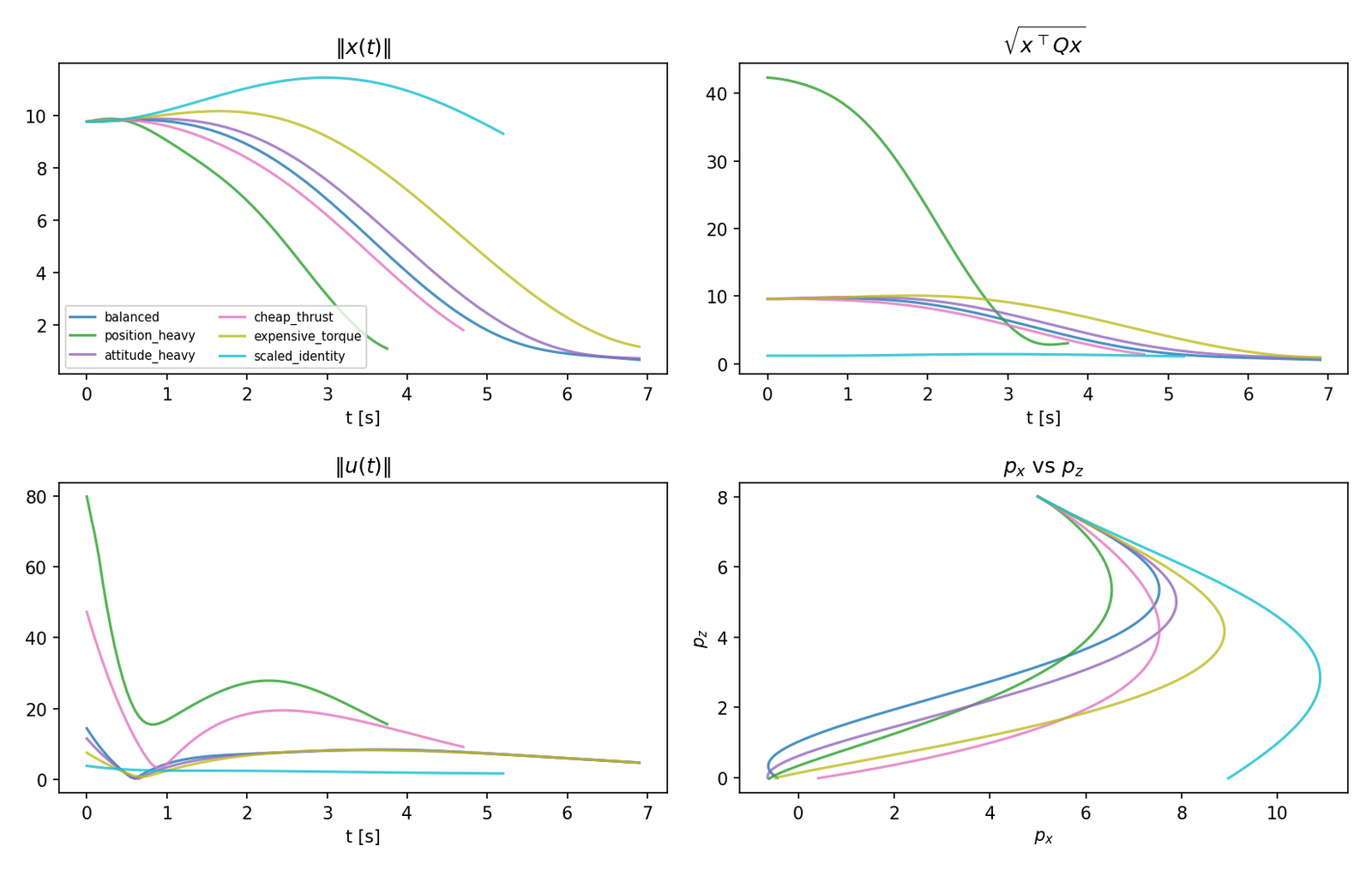
Heuristic presets were swept on the hover LTI plant to reflect the underlying control intuition: pos_heavy and att_heavy tighten position and attitude transients at the cost of higher $\int u^{\top}Ru\,dt$; cheap_th and exp_trq isolate thrust- versus torque-dominated effort; balanced is the baseline used in later parts.
| Preset | $Q = \mathrm{diag}(\cdot)$ | $R$ | $Q_f = \mathrm{diag}(\cdot)$ |
|---|---|---|---|
balanced |
(1, 1, 0.5, 0.5, 10, 5, 0.01) | (0.1, 1) | (10, 10, 1, 1, 50, 20, 0.1) |
pos_heavy |
(20, 20, 2, 2, 5, 2, 0.01) | (0.1, 1) | (50, 50, 5, 5, 20, 10, 0.1) |
att_heavy |
(1, 1, 0.5, 0.5, 50, 25, 0.01) | (0.1, 2) | (10, 10, 1, 1, 100, 50, 0.1) |
cheap_th |
(1, 1, 0.5, 0.5, 10, 5, 0.01) | (0.01, 1) | (10, 10, 1, 1, 50, 20, 0.1) |
exp_trq |
(1, 1, 0.5, 0.5, 10, 5, 0.01) | (0.1, 10) | (10, 10, 1, 1, 50, 20, 0.1) |
scaled_id |
(10⁻², 10⁻², 0.04, 0.04, 25, 4, 1) | (1, 1) | same as $Q$ |
Controllability Analysis
Two complementary tools were used. The algebraic controllability matrix checks structural control authority for a frozen-time snapshot of the plant; with $n = 7$ states,
\[\mathcal{C} = \begin{bmatrix} B & AB & A^2B & \cdots & A^6B \end{bmatrix} \in \mathbb{R}^{7 \times 14}\]The finite-horizon controllability Gramian quantifies how expensive that authority is:
\[W_c(0,t_f) = \int_0^{t_f} \Phi(0,\tau)B(\tau)B(\tau)^{\top}\Phi(0,\tau)^{\top}\,d\tau\]Rather than form the state transition matrix explicitly, $W_c$ is computed by integrating its differential form, and the minimum control energy required to reach a state deviation $x_f$ follows directly:
\[\dot{W_c}(t) = A(t)W_c(t) + W_c(t)A(t)^{\top} + B(t)B(t)^{\top}, \qquad E = x_f^{\top}W_c^{-1}x_f\]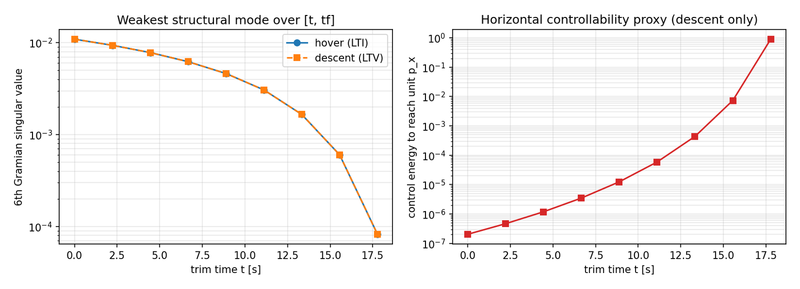
| Model | rank($\mathcal{C}$) | $\sigma_1$ | $\sigma_6$ | $\sigma_7$ |
|---|---|---|---|---|
| Hover LTI ($t = 0$ s) | 7/7 | 0.98 | 0.0489 | 0 |
| Descent LTV ($t = 0$ s) | 7/7 | 0.98 | 0.0489 | 0 |
| Hover LTI ($t = 15$ s) | 7/7 | 0.98 | 0.0489 | 0 |
| Descent LTV ($t = 15$ s) | 7/7 | 0.98 | 0.1 | 0 |
Both trims are algebraically full rank, but rank alone is misleading. Controllable energy in the weakest meaningful mode shrinks as $t_f - t$ shrinks, especially for horizontal motion. The descent LTV plant at $t = 15$ s shows larger $B$-column entries for $v_z$ and weaker indirect authority on $p_x$ — horizontal acceleration enters only through attitude coupling — which is the physical origin of the “weakly controllable” label.
Analysis
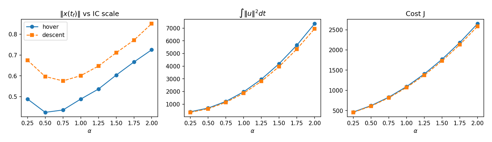
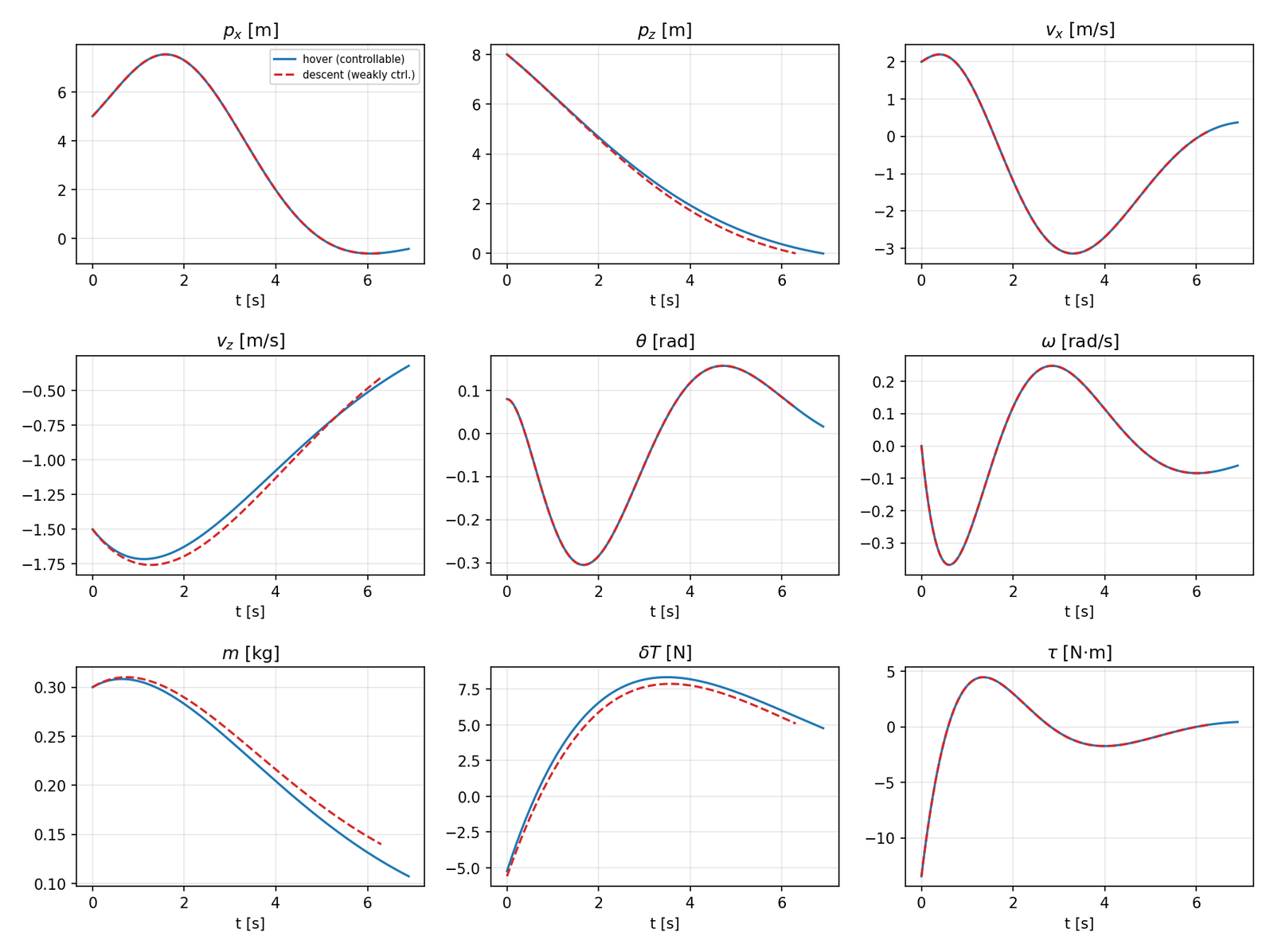
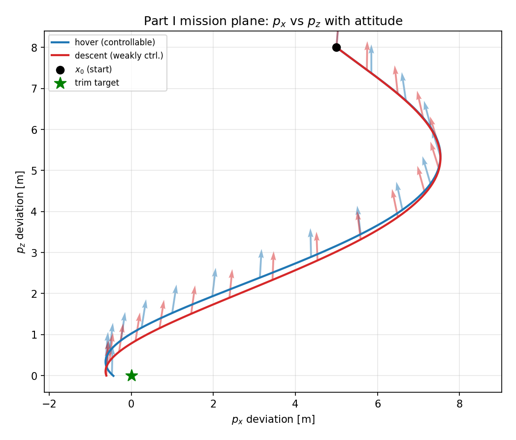
At small perturbations, descent can perform worse — a weak plant combined with the wrong linearization point. At large perturbations hover overtakes it, since the hover LTI model may be overly optimistic at large scaling $\alpha$: the linear model stays fixed while the state explores larger deviations.
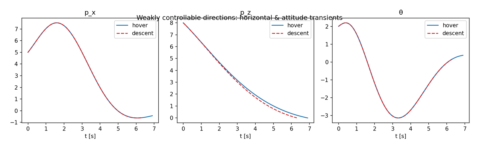
Swings in $p_x$ and $\theta$ indicate structural difficulty; even the nominally controllable hover trim struggles, which the Gramian analysis had already flagged as expensive to correct. The gap between trims is clearest in $p_z$, driven by the mass/thrust schedule and the changing trim point.
Validation
Because this phase uses the Riccati sweep rather than a shooting solver, optimality is validated by verifying the backward-pass terminal conditions and forward-pass tracking convergence.
| Metric | Target | Computed |
|---|---|---|
| $\lVert P(t_f) - Q_f \rVert_\infty$ | 0 | 1.22 × 10⁻¹⁴ |
| $\lVert e(t_f) \rVert_\infty$ | 0 | 4.51 × 10⁻⁶ |
V. Part II — Optimal Trajectory Tracking
Deviation from base: the running cost penalizes deviation from a reference, $(x - x_{\text{ref}})^{\top}Q(x - x_{\text{ref}})$, and there is no terminal cost. The first change makes the costate equation affine rather than linear; the second sends the terminal costate to zero.
Formulation
\[J = \int_0^{t_f}\left[(x-x_{\text{ref}})^{\top}Q(x-x_{\text{ref}}) + u^{\top}Ru\right]dt\]The Hamiltonian and stationarity condition carry over unchanged. Only the adjoint equation picks up the reference term, and transversality collapses:
\[\dot{p} = -2Q(x - x_{\text{ref}}) - A^{\top}p, \qquad p(t_f) = \left.\frac{\partial \varphi}{\partial x}\right|_{t_f} = 0 \quad (\varphi \equiv 0)\]Why the Riccati Substitution Must Be Extended
The forcing term $2Qx_{\text{ref}}$ is independent of $x$, so the pure ansatz $p = Px$ can no longer absorb it — a linear-in-$x$ form cannot represent an affine equation. The substitution is therefore augmented with an auxiliary vector:
\[p(t) = P(t)x(t) + s(t)\]Repeating the base derivation with this ansatz and grouping terms gives two brackets, one proportional to $x(t)$ and one constant:
\[\underbrace{\left[\dot{P} + PA + A^{\top}P - \tfrac{1}{2}PBR^{-1}B^{\top}P + 2Q\right]}_{\text{identical to base case}}x(t) + \underbrace{\left[\dot{s} + A^{\top}s - \tfrac{1}{2}PBR^{-1}B^{\top}s - 2Qx_{\text{ref}}\right]}_{\text{new}} = 0\]Both brackets must vanish independently. The first recovers the same Riccati equation as Part I; the second is new:
\[\dot{s} = -\left(A^{\top} - \tfrac{1}{2}PBR^{-1}B^{\top}\right)s + 2Qx_{\text{ref}}\]Since $p(t_f) = P(t_f)x(t_f) + s(t_f) = 0$ must hold for an arbitrary terminal state, both pieces integrate backward from homogeneous terminal conditions $P(t_f) = 0$, $s(t_f) = 0$, reflecting the absence of any terminal penalty.
Substituting back splits the control cleanly into feedback and feedforward:
\[u^{*}(t) = -\tfrac{1}{2}R^{-1}B^{\top}P(t)x(t) - \tfrac{1}{2}R^{-1}B^{\top}s(t) \;=\; -K(t)x(t) + u_{ff}(t)\]$K(t)x(t)$ stabilizes the vehicle and kills deviations; $u_{ff}(t)$ anticipates the control effort the reference itself demands.
Scenario
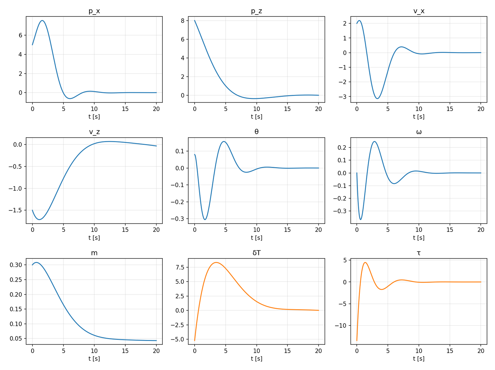
The reference $x_{\text{ref}}(t)$ is one of the optimal regulation trajectories recorded in Part I — a damped maneuver settling to hover trim. To produce a nontrivial transient, the controller is initialized at
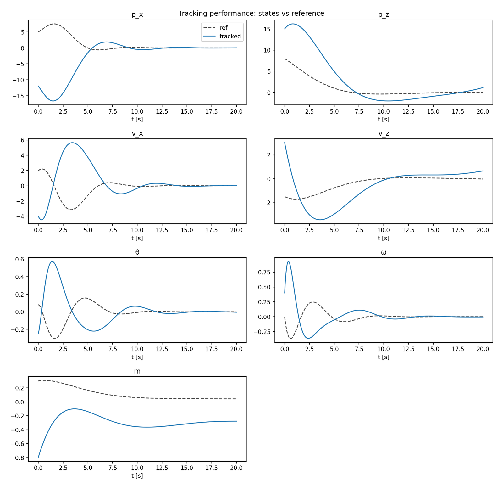
\[x_0^{\text{trk}} = \begin{bmatrix} -12 & 15 & -4 & 3 & -0.25 & 0.4 & -0.8 \end{bmatrix}^{\top}\]deviating from the reference start by $\Delta p_x \approx 17$ m and $\Delta\theta \approx 0.33$ rad. Because the hover linearization is altitude-invariant ($p_z$ is decoupled and absent from every right-hand side), the maneuver is executed about a hover point $h = 12$ m above the pad; this leaves $A$, $B$, $x_{\text{ref}}$, and the feedback law unchanged while the absolute altitude $p_z = h + p_z^{\text{dev}}$ enforces the ground constraint. Minimum absolute altitude is 11.6 m (reference) and 10.0 m (tracker), with mass margin above 12 kg throughout.
Analysis
The tracker starts with state error $\lVert e(0) \rVert \approx 19.9$, peaks at $\lVert e \rVert \approx 26.2$ near $t = 1.6$ s as it first accelerates toward the reference, and the cost-weighted error decays to within 10% of its peak by $t \approx 6.9$ s. The residual terminal error $\lVert e(t_f) \rVert \approx 1.38$ is concentrated in the vertical and mass channels ($\lvert e_{p_z} \rvert \approx 1.16$, $\lvert e_{v_z} \rvert \approx 0.67$, $\lvert e_m \rvert \approx 0.32$), while horizontal and attitude errors are driven to $O(10^{-3})$.
This residual is an expected feature of the fixed-horizon, free-final-state problem with no terminal cost. As $t \to t_f$, both $K(t)$ and $s(t)$ decay, so the controller “relaxes” near $t_f$ and the weakly penalized vertical/mass states drift slightly.
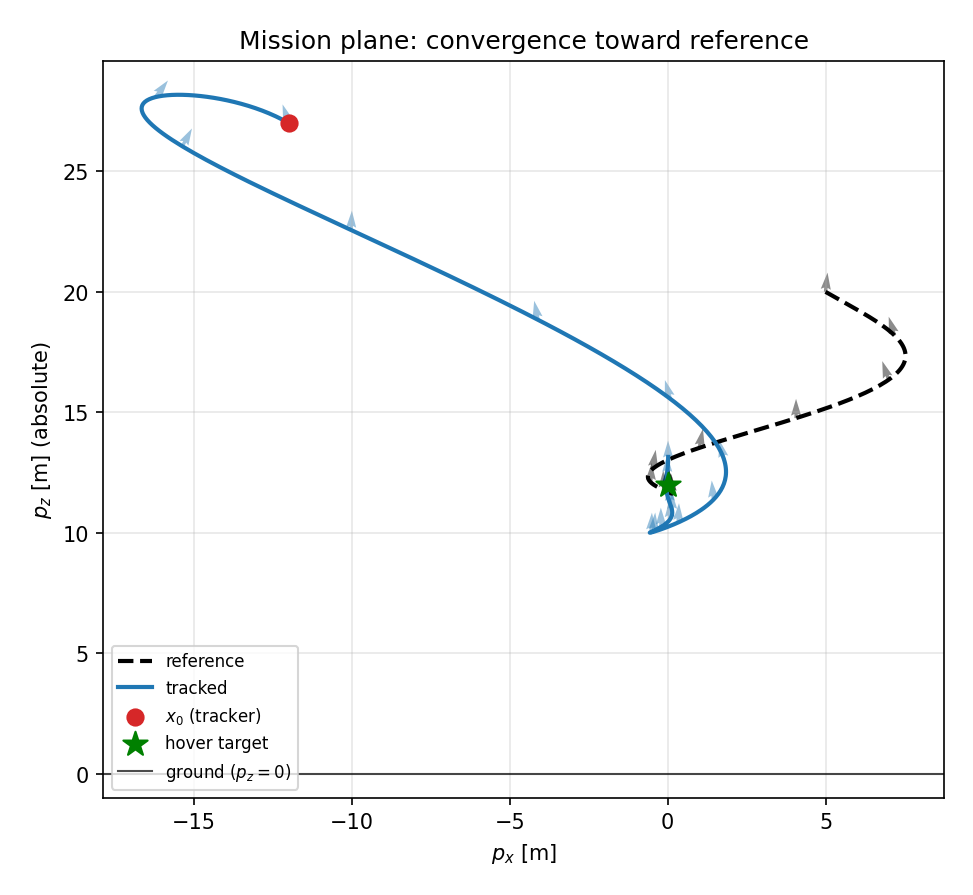
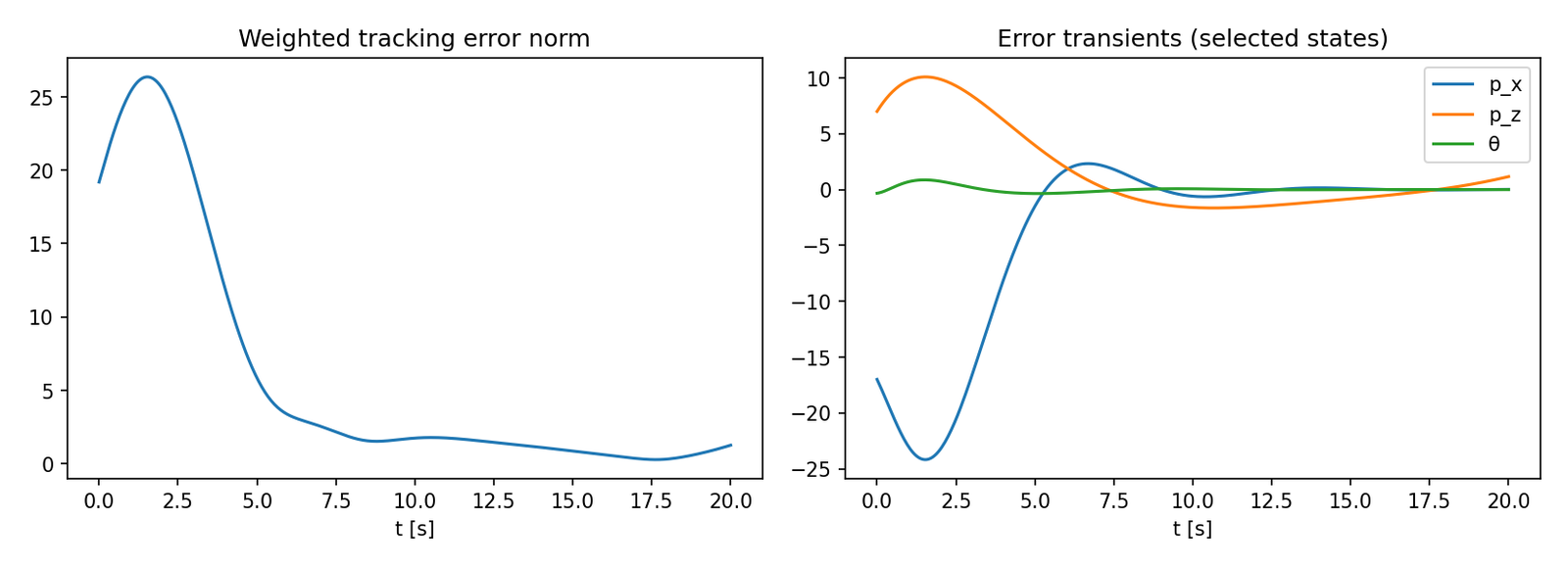
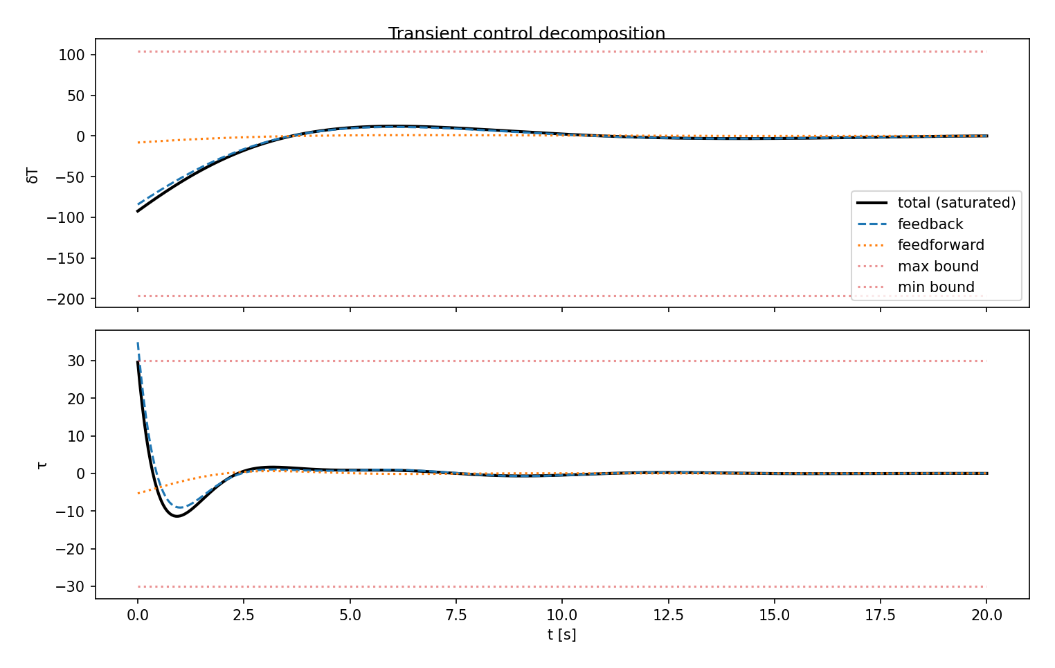
Scalar tracking error decays monotonically in the weighted norm. Because the target is moving rather than zero, there is no mid-horizon rebound; position errors decay slowly and dominate, while attitude error stays small throughout. The control splits as $u^{*}(t) = -K(t)e(t) + u_{ff}(t)$, with the feedback term dominating the transient and the feedforward term small and slowly varying, since the reference is itself a decaying signal. The torque channel uses nearly full authority at $t = 0$ ($\tau \approx 29.6$ N·m against the ±30 N·m bound) to arrest attitude error, but no channel saturates over the horizon.
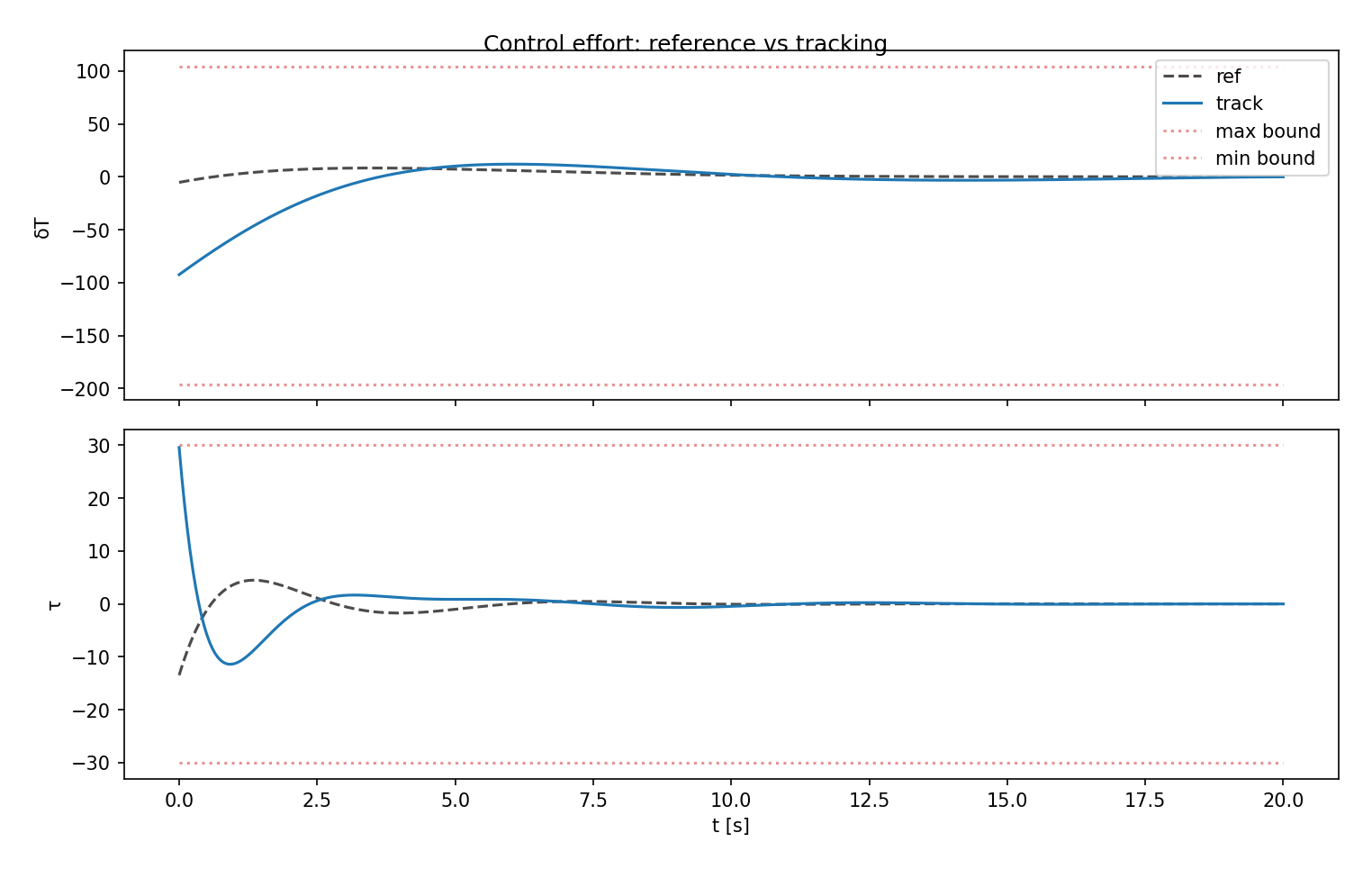
Relative to the smooth reference plan, rejoining from the displaced initial state is expensive: the tracker expends $\int u^{\top}Ru\,dt \approx 1041$ versus $\approx 86$ for the reference, a 12× increase concentrated in the first few seconds. Peak thrust deviation reaches $\delta T \approx 92$ N, within the +104 N headroom to $T_{\max}$, confirming that the chosen weights keep the catch-up maneuver feasible without thrust saturation. Once error is nulled, the tracking control collapses onto the reference control.
Robustness
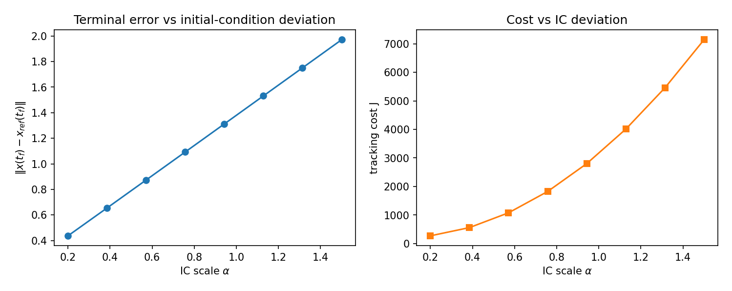
Sweeping the initial offset by a factor $\alpha$ confirms the structure of the linear tracking law: terminal error grows essentially linearly in $\alpha$ (slope $\approx 1.18$), consistent with superposition of the closed-loop transition map, while tracking cost grows quadratically, since the cost is a quadratic form in the deviation. There is no threshold or instability over the tested range — the degradation is graceful.
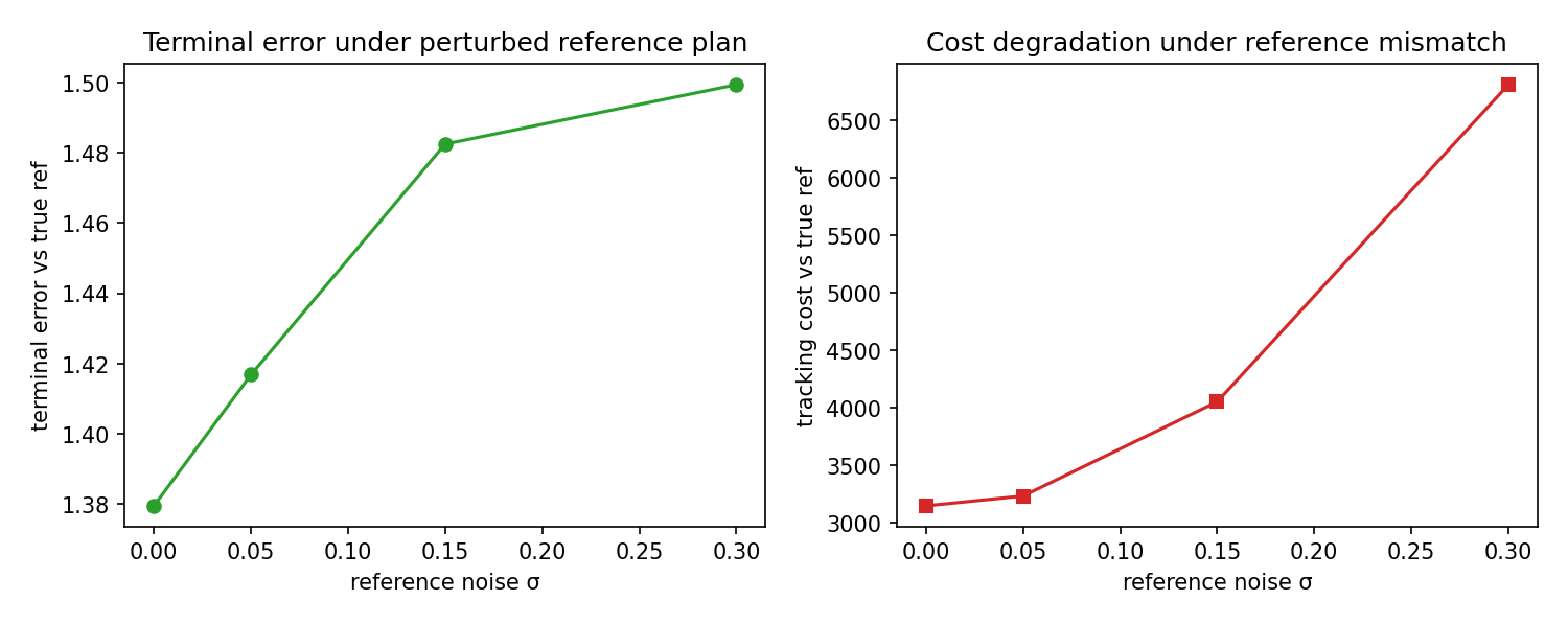
Corrupting the reference used to build the feedforward with zero-mean noise of level $\sigma$ tells a different story. Terminal error is only mildly affected (1.38 at $\sigma = 0$ to 1.50 at $\sigma = 0.30$) because the feedback term rejects high-frequency reference error, but tracking cost degrades markedly (≈3150 to ≈6810, a 2.2× increase) as the controller wastes effort chasing a corrupted plan.
This exposes a structural limitation: the law is non-causal. $s(t)$ comes from a backward integration requiring the entire future $x_{\text{ref}}(\tau)$ on $[t, t_f]$. Without that preview only $u = -K(t)e(t)$ remains — stable, but lagging and costlier. A causal fix would replan online (receding-horizon MPC) or generate $x_{\text{ref}}$ from a predictive model.
Validation
Because Part II has no terminal cost and a free final state, optimality is certified against the PMP necessary conditions rather than terminal convergence.
| Metric | Target | Computed |
|---|---|---|
| $\lVert P(t_f) \rVert_\infty$ (Riccati terminal) | 0 | 1.0 × 10⁻¹⁴ |
| $\lVert s(t_f) \rVert_\infty$ (feedforward terminal) | 0 | 1.6 × 10⁻¹⁷ |
| $\max_t \lVert Ru + B^{\top}\lambda \rVert$ (stationarity) | 0 | 1.1 × 10⁻¹⁴ |
The terminal tracking error is not required to vanish for this free-final-state problem; its value is a result, not a residual.
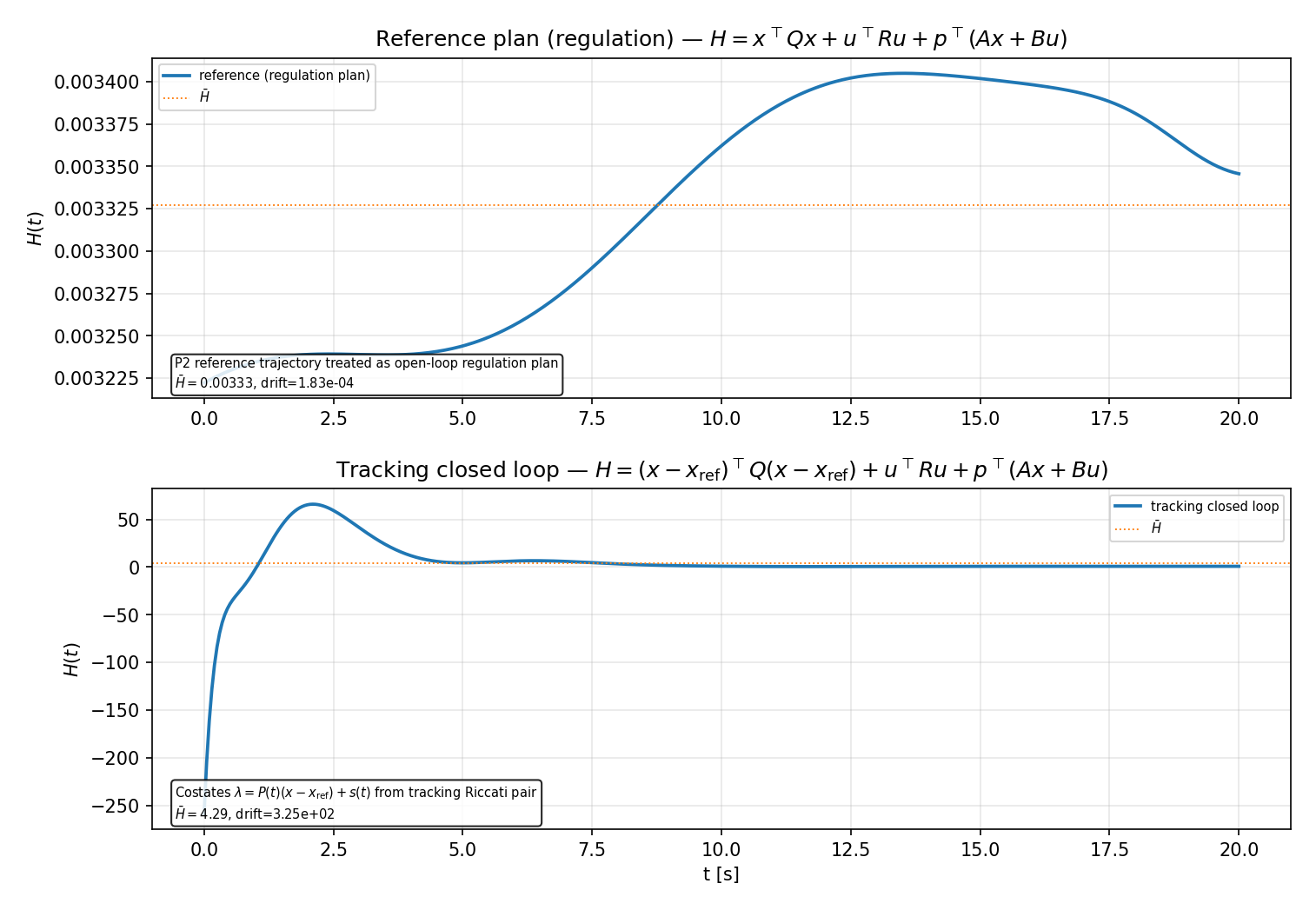
For the autonomous reference plan $H$ is constant to $\sim 10^{-4}$, whereas for the tracking problem $H$ is intentionally time-varying: explicit dependence on $x_{\text{ref}}(t)$ makes $\partial H/\partial t \neq 0$. The relevant optimality certificate for tracking is therefore the stationarity/costate residual, not constancy of $H$.
VI. Part III — The Mission Problem
Deviation from base: the final time becomes free, which adds the closure condition $H(t_f) = 0$. Phase A additionally strips $u$ out of the cost entirely; Phase B additionally constrains the endpoint to a manifold, which adds multiplier terms to transversality.
The mission is two-phase: a minimum-time ascent to a rendezvous state, followed by an optimal return-and-land.
Phase A — Minimum-Time Ascent
\[J_A = \int_0^{t_1} 1\,dt = t_1\]With $L = 1$, the Hamiltonian loses all $u$-dependence in the cost:
\[H_A = 1 + p^{\top}Ax + p^{\top}Bu, \qquad \dot{p} = -A^{\top}p\]This is the structural break. $\partial H_A/\partial u = B^{\top}p$ is now independent of $u$, so stationarity cannot solve for $u^{*}$ — there is no interior minimum. Minimizing $H$ pointwise instead drives each channel to whichever bound reduces $H$, governed by the switching function $S(t) = B^{\top}p(t)$:
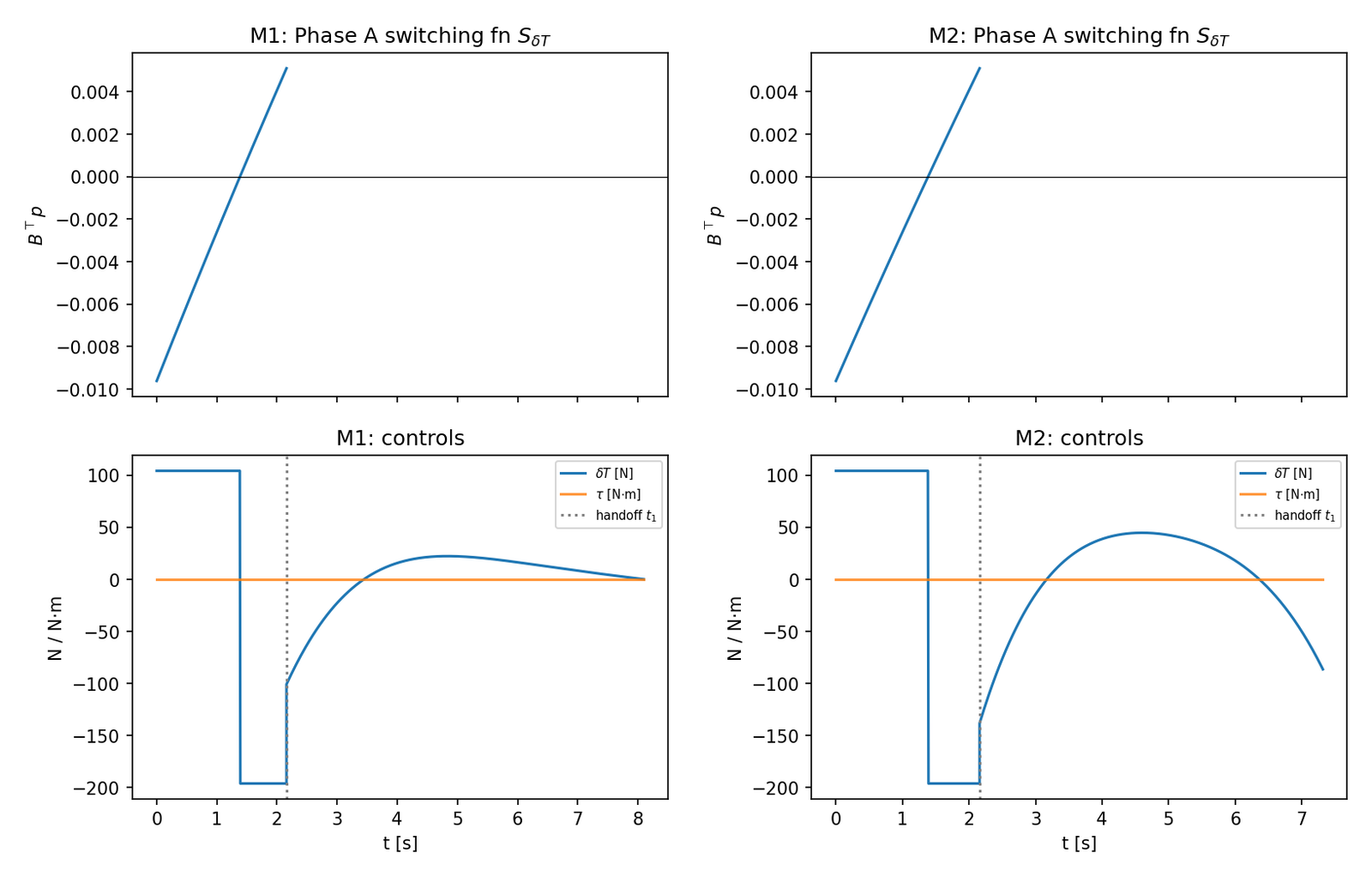
\[u_i^{*}(t) = \begin{cases} U_{\max,i} & \text{if } S_i(t) < 0 \\ U_{\min,i} & \text{if } S_i(t) > 0 \end{cases}\]The control is bang–bang. No singular arcs arise on thrust, since $S_{\delta T}$ has one sign change. The torque channel is structurally singular for vertical ascent ($S_\tau = p_\omega/I \equiv 0$ with $\theta = \omega = 0$), so $\tau^{*} = 0$ throughout.
The ascent drives the vehicle to a prescribed rendezvous state with the first six components fixed at $t_1$ and terminal mass left free, so the corresponding costate vanishes by transversality. Because $t_1$ is free, the minimum-time condition closes the system:
\[x_i(t_1) = x_{\text{sky},i},\ \ i \in \{p_x,p_z,v_x,v_z,\theta,\omega\}, \qquad p_m(t_1) = 0, \qquad H_A(t_1) = 0\]Note that $H_A \equiv 0$ holds along the entire arc, not just at $t_1$ — a useful numerical check.
Implementation. Phase A is solved by indirect single shooting in mission.py. The decision vector is $Z = [p(0);\, t_1] \in \mathbb{R}^8$; each candidate is propagated forward with solve_ivp (RK45) on the 14-dimensional state–costate system using the bang–bang law, and the eight residuals are driven below $10^{-5}$ by scipy.optimize.least_squares with 12 random multi-starts and $t_1 \in [0.3, 5]$ s. The rendezvous is $x_{\text{sky}} = (0, 8, 0, v_{z,\text{sky}}, 0, 0, 0)^{\top}$ in hover-deviation coordinates, with $v_{z,\text{sky}} \in {-2, 0, +2}$ m/s for the terminal-velocity comparison.
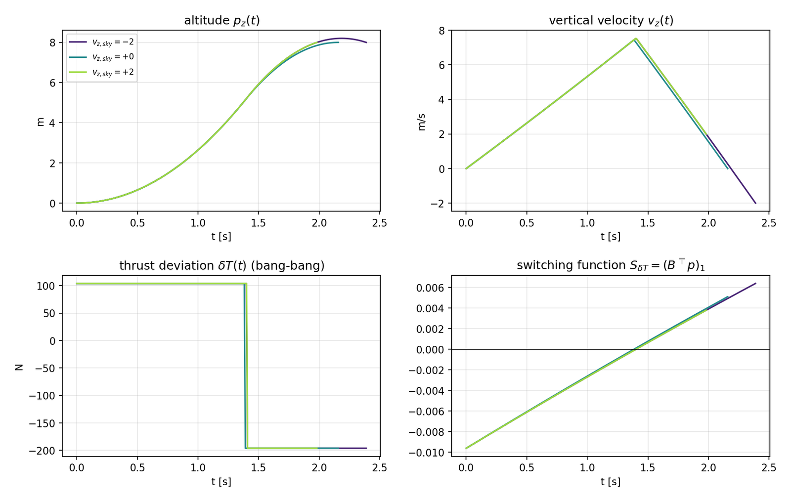
Every case exhibits exactly one thrust switch: maximum $\delta T$ accelerates upward until $S_{\delta T}$ changes sign, then minimum thrust completes the rendezvous. Thrust saturates because time appears linearly in $J_A$ with no control penalty. Ascent time depends strongly on $v_{z,\text{sky}}$ — $t_1 = 2.39$, 2.16, and 1.98 s for −2, 0, and +2 m/s — and the switch occurs late in the arc (≈59–71% of $t_1$), so deceleration to target speed is back-loaded. Propellant use is nearly unchanged (≈2.08 kg) because the maneuver is short; mass depletion over ~2 s is too small to materially change $1/m$ and control authority.
Phase B — Return and Land
Phase B begins where Phase A ends, so $x(0) = x_1$. The cost returns to quadratic form, which means the unconstrained control law and adjoint equations are identical to Part I:
\[J_B = \int_0^{t_f}\left(x^{\top}Qx + u^{\top}Ru\right)dt, \qquad u^{*} = -\tfrac{1}{2}R^{-1}B^{\top}p, \qquad \dot{p} = -2Qx - A^{\top}p\]Two things change. First, $t_f$ is free, so PMP imposes $H_B(t_f) = 0$. Second — and this is the substantive addition — the endpoint is confined to a manifold, so transversality gains a multiplier term for each active constraint:
\[p(t_f) = \left.\frac{\partial \varphi}{\partial x}\right|_{t_f} + \sum_j \nu_j \nabla h_j(x(t_f))\]The interpretation is geometric: the terminal costate is free to have any component normal to the manifold (absorbed by the multipliers) but is pinned in every direction tangent to it.
Manifold 1 — pinpoint landing on flat ground.
\[h_1 = p_z = 0, \qquad h_2 = v_z = 0, \qquad h_3 = \theta = 0\]The gradients are the corresponding unit vectors, so each constrained costate simply picks up its own multiplier, and the four unconstrained costates ($p_{p_x}, p_{v_x}, p_\omega, p_m$) reduce to $\partial\varphi/\partial x$.
Manifold 2 — landing on a circular platform. The altitude fix is replaced by a sphere:
\[h_1 = (p_x - p_c)^2 + p_z^2 - r^2 = 0, \qquad h_2 = v_z = 0, \qquad h_3 = \theta = 0\]Now $\nabla h_1 = [2(p_x - p_c),\ 2p_z,\ 0,0,0,0,0]^{\top}$ couples $p_x$ and $p_z$, spanning two dimensions instead of one:
\[p_{p_x}(t_f) = \frac{\partial\varphi}{\partial p_x} + 2\nu_1(p_x(t_f) - p_c), \qquad p_{p_z}(t_f) = \frac{\partial\varphi}{\partial p_z} + 2\nu_1 p_z(t_f)\]The unknown multiplier $\nu_1$ is eliminated by dividing these two equations (with $\partial\varphi/\partial x = 0$), which yields a clean collinearity condition passed directly to the solver:
\[\frac{p_{p_x}(t_f)}{p_{p_z}(t_f)} = \frac{p_x(t_f) - p_c}{p_z(t_f)}\]Physically: the position costate must align with the outward normal of the sphere at touchdown.
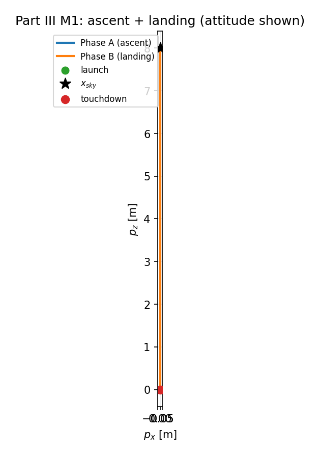
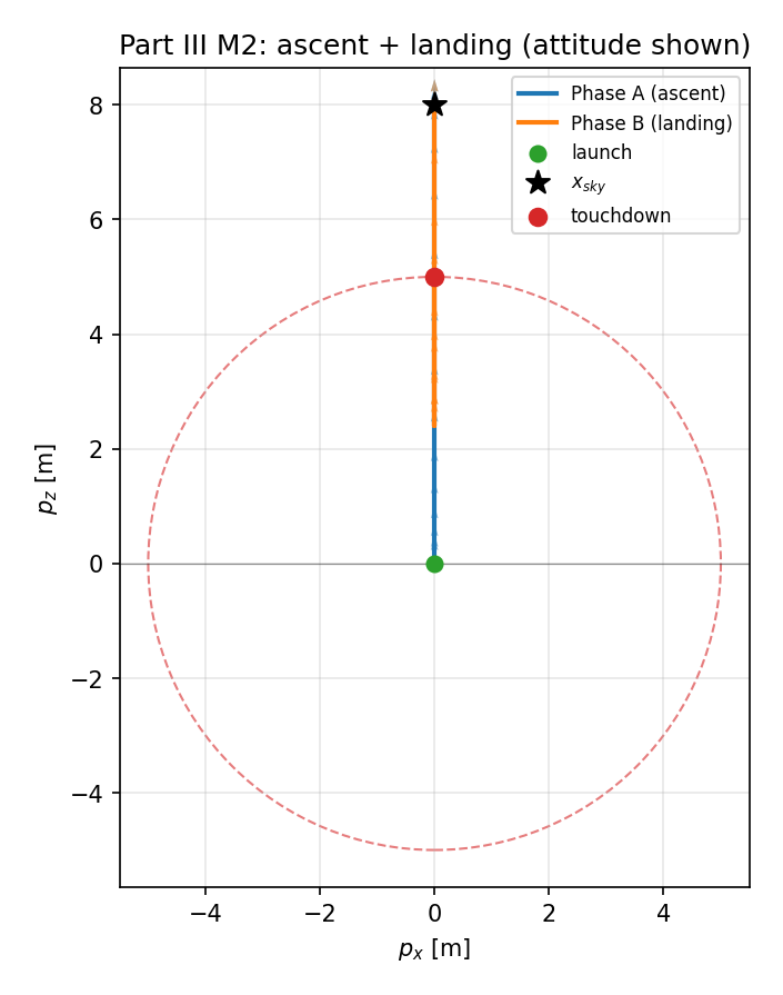
Implementation. The combined state–costate system with the saturated stationarity law is mapped onto $s \in [0,1]$ via $t = t_1 + s(t_f - t_1)$, with the unknown duration entering as a free parameter. The split boundary conditions are the handoff $x(t_1) = x_1$, seven manifold endpoint and transversality residuals, and the free-time closure $H_B(t_f) = 0$ — fifteen conditions for fourteen states plus the parameter. The platform is centred at $(p_c, 0) = (0,0)$ so that M1 lands at $(0,0)$ and M2 at the apex $(0,r)$, sharing the same horizontal footprint and isolating the effect of manifold geometry.
Manifold Comparison
| Metric | M1 (flat) | M2 (platform) |
|---|---|---|
| Ascent time $t_1$ [s] | 2.158 | 2.158 |
| Landing time $t_f$ [s] | 8.097 | 7.315 |
| Phase B energy $\int u^{\top}Ru\,dt$ | 215.7 | 526.2 |
| Touchdown $(p_x, p_z)$ [m] | (0, 0) | (0, 5) |
| Shooting $\lVert \text{res} \rVert_\infty$ | 6.2 × 10⁻⁸ | 6.2 × 10⁻⁸ |
| Terminal manifold $\lVert \text{res} \rVert_\infty$ | 7.0 × 10⁻²¹ | 1.1 × 10⁻¹⁴ |
| $H_A$ drift (min-time, ≡ 0) | 2.9 × 10⁻⁹ | 2.9 × 10⁻⁹ |
| $H_B$ drift (free-time, ≡ 0) | 9.7 × 10⁻¹² | 9.6 × 10⁻¹¹ |
| Min. altitude $p_z$ [m] | 0.000 | 0.000 |
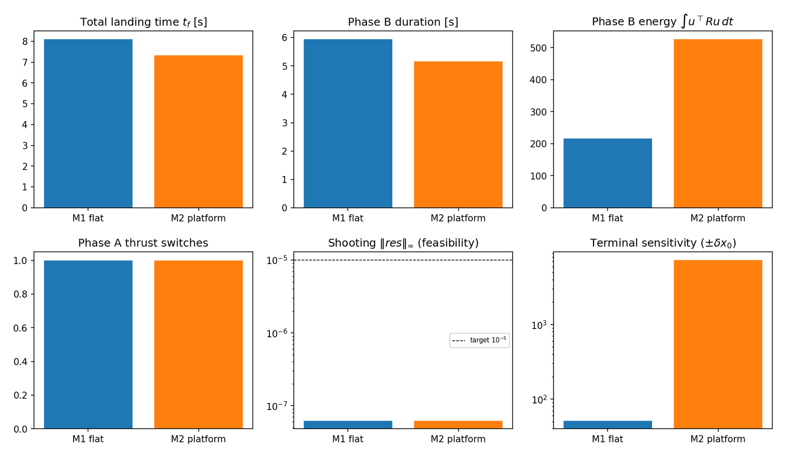
Landing time. M2 completes sooner — 7.32 s versus 8.10 s — because touchdown at the platform apex $(0,5)$ m avoids the long final vertical flare required to reach $p_z = 0$ on flat ground.
Energy. Despite the shorter clock time, M2 costs ≈2.4× more control energy. The lofted descent arc and stronger horizontal–vertical coordination dominate the budget.
Switching structure. Phase A is identical in both cases. Phase B uses smooth saturated costate feedback in both manifolds — no further bang–bang arcs — with M2 displaying larger mid-descent $\delta T$ and $\tau$ activity to steer onto the curved approach.
Terminal sensitivity. Perturbing the handoff state by ±0.05 on each component raises the worst-case terminal residual to ~51 for M1 but ~1.9 × 10³ for M2. The sphere constraint and collinearity condition tightly couple position and costate at touchdown, making M2 far more sensitive.
The geometric explanation ties it together: M1’s flat manifold allows a nearly vertical descent, while M2’s sphere forces a bowed trajectory that must intercept the surface along its outward normal. Transversality requires the position costate to align with that normal, which demands sustained lateral thrust and attitude correction through Phase B.
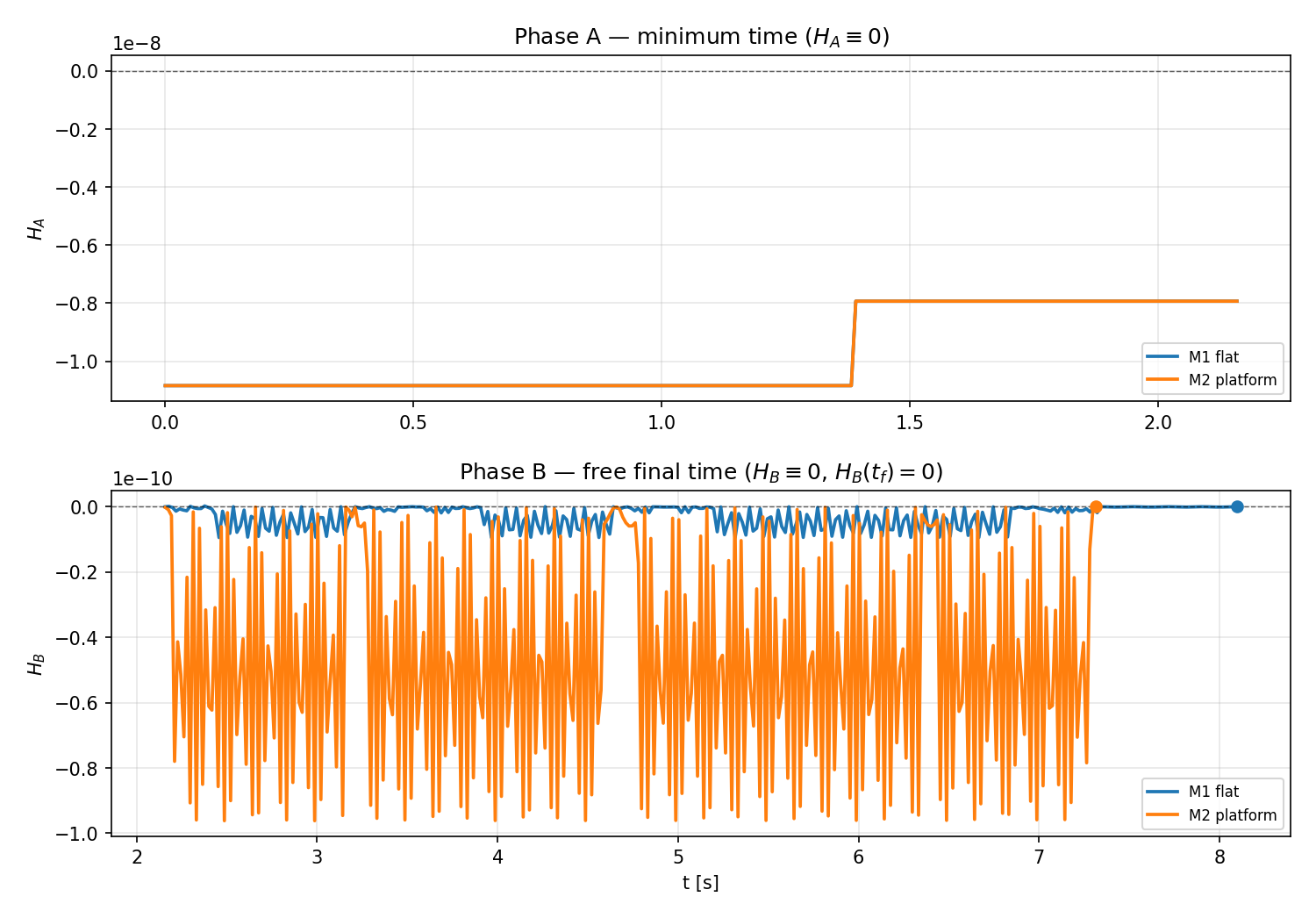
Both phases are free-final-time problems, so PMP requires the Hamiltonian to vanish identically rather than merely stay constant. Phase A holds $H_A \equiv 0$ to $O(10^{-9})$ and Phase B holds $H_B \equiv 0$ to $O(10^{-11})$, confirming the free-time transversality closure in both manifolds.
VII. Part IV — Nonlinear Optimal Control Near Hover
Deviation from base: the plant is the full nonlinear model. The Riccati substitution assumed linear dynamics and is now invalid; the coupled 14-state TPBVP must be solved directly.
Formulation
\[\min_u \int_0^{t_f}\left(x^{\top}Qx + u^{\top}Ru\right)dt\]subject to the nonlinear EOM of Section I, anchored at a known $x(0) = x_0$. Adjoining the nonlinear dynamics with costate $p$:
\[H = x^{\top}Qx + u^{\top}Ru + p_1 v_x + p_2 v_z - p_3\frac{T}{m}\sin\theta + p_4\left(\frac{T}{m}\cos\theta - g\right) + p_5\omega + p_6\frac{\tau}{I} - p_7\alpha T\]The adjoint equations follow from $\dot{p} = -\partial H/\partial x$. Unlike the linear case they are no longer a fixed matrix product — the attitude and mass channels pick up genuine coupling:
\[\begin{aligned} \dot{p}_1 &= -2Q_{11}p_x & \dot{p}_5 &= -2Q_{55}\theta + \frac{T}{m}\left(p_3\cos\theta + p_4\sin\theta\right) \\ \dot{p}_2 &= -2Q_{22}p_z & \dot{p}_6 &= -2Q_{66}\omega - p_5 \\ \dot{p}_3 &= -2Q_{33}v_x - p_1 & \dot{p}_7 &= -2Q_{77}m + \frac{T}{m^2}\left(p_4\cos\theta - p_3\sin\theta\right) \\ \dot{p}_4 &= -2Q_{44}v_z - p_2 \end{aligned}\]The $\dot{p}_5$ and $\dot{p}_7$ equations are where the nonlinearity lives: pitch feeds back through the thrust resolution, and mass feeds back through $T/m^2$.
Stationarity still gives closed-form controls, now saturated to the actuator bounds expressed in deviation form:
\[\delta T^{*} = \mathrm{sat}\left[\frac{1}{2R_{11}}\left(p_3\frac{\sin\theta}{m} - p_4\frac{\cos\theta}{m} + p_7\alpha\right)\right], \qquad \tau^{*} = \mathrm{sat}\left[-\frac{p_6}{2IR_{22}}\right]\]Substituting these back into the 7 state and 7 adjoint equations creates a deeply coupled system of 14 nonlinear first-order ODEs, solved simultaneously on $t \in [0, t_f]$ subject to split boundary conditions $x(0) = x_0$ and $p(t_f) = 2Q_f x(t_f)$.
Numerical Implementation
The problem is solved in hover-deviation coordinates so the linearized solutions of previous parts serve directly as the nonlinear warm start. Three scenarios share a common $x_0 = [1,\ 1.5,\ 0.4,\ -0.25,\ 0.12,\ 0,\ 0.05]^{\top}$ and horizon:
- LQR on the linear plant — backward Riccati sweep from Part I, integrated forward on $\dot{x} = Ax + Bu$.
- LQR on the nonlinear plant — the same time-varying gain applied to the full nonlinear EOM with fixed-step RK4 and clipped control. This isolates the modeling error incurred by using a linear law on the true plant.
- Nonlinear PMP / TPBVP — the coupled 14-state system solved by collocation with control substituted in closed form from stationarity.
Restriction to near-hover. True hover is not an equilibrium of a variable-mass vehicle — holding $T = mg$ continuously depletes mass at $\dot{m} = -\alpha m g$ — so the horizon is kept short at $t_f = 4$ s with 201 uniform nodes. This keeps the trajectory near hover and the mass safely above $m_{\text{dry}}$.
Warm start and costate scaling. The collocation guess uses the Scenario 1 state history with costate guess $p(t) = 2P(t)x(t)$; the factor of two maps the $\tfrac{1}{2}$-scaled Riccati costate to the un-scaled running cost used here. Convergence is declared at a collocation tolerance of $10^{-6}$.
Analysis
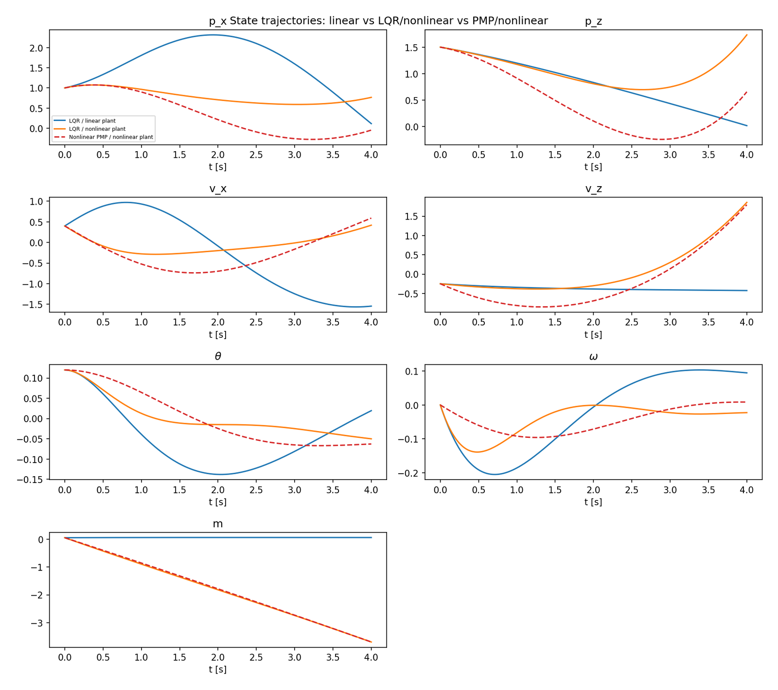
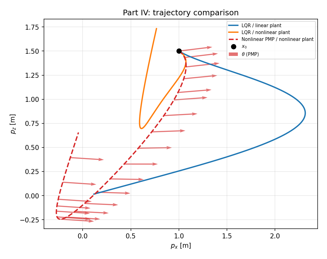
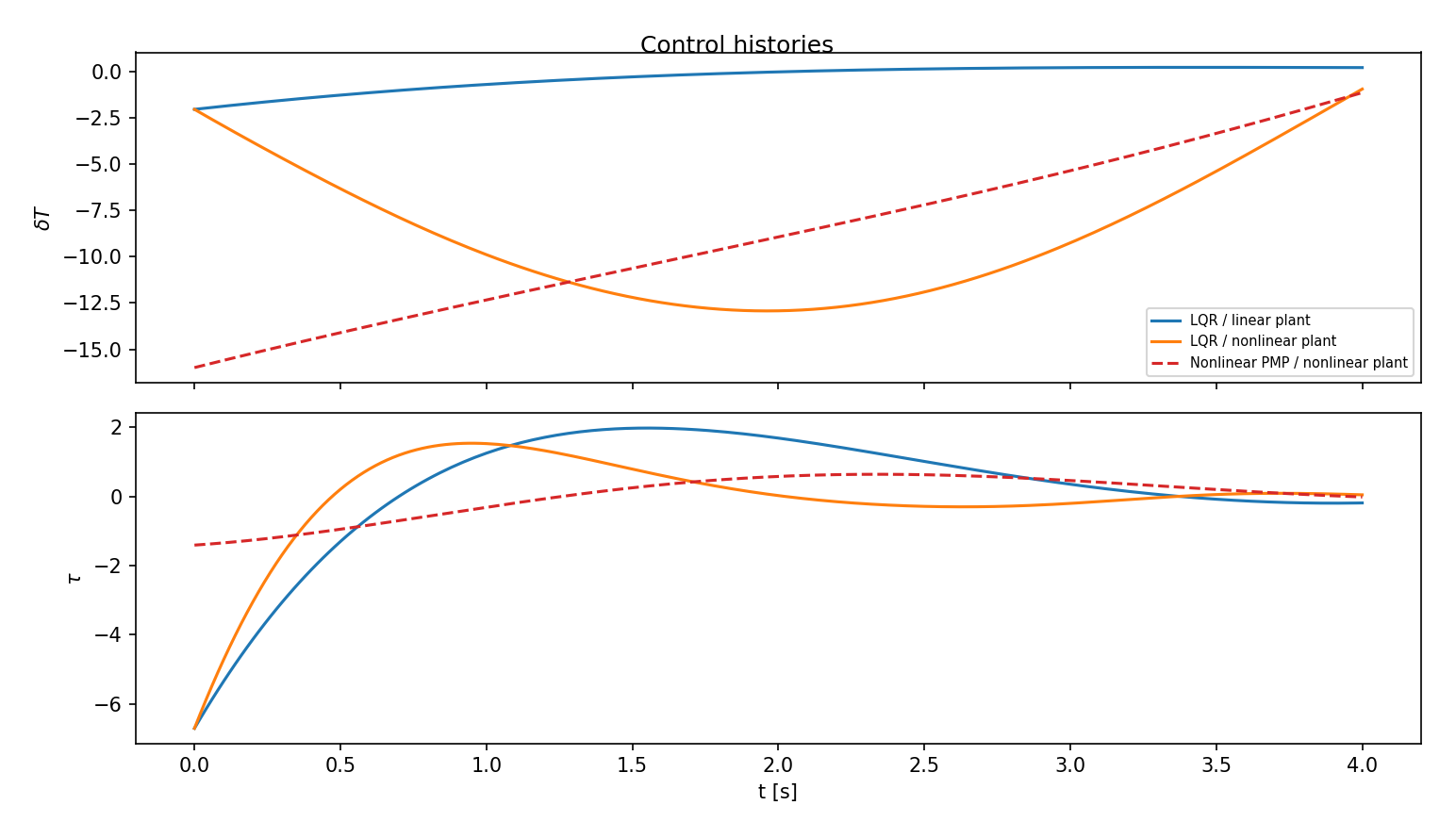
Scenarios (1) and (2) agree early but diverge as $\theta$ and $m$ evolve; the nonlinear PMP solution trims peak $p_z$ and $\theta$ by exploiting the $\sin\theta$ and $T/m$ coupling that the linear law cannot see. The linear law over-commands on the true plant, raising control effort $J_u$ from 13.2 to 42.9, while PMP recovers 39.4 (≈8% savings) and lowers total $J$ by 41% versus Scenario 2.
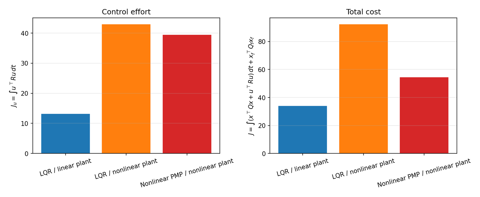
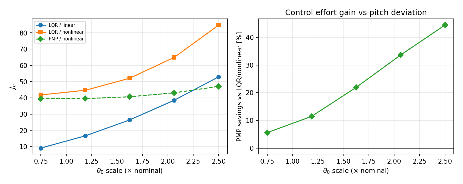
Terminal norms tighten under PMP, collocation converges in few refinements from the LQR seed, and the PMP advantage grows with initial pitch. The linear approximation remains accurate for small attitude and mass deviations over 4 s; it breaks down once thrust–gravity resolution and mass depletion accumulate.
Validation
Part IV is a fixed-final-time, free-endpoint problem with autonomous hover-trim dynamics, so the Hamiltonian must remain constant along the optimal trajectory — but unlike the free-final-time mission of Part III, that constant is not required to vanish.
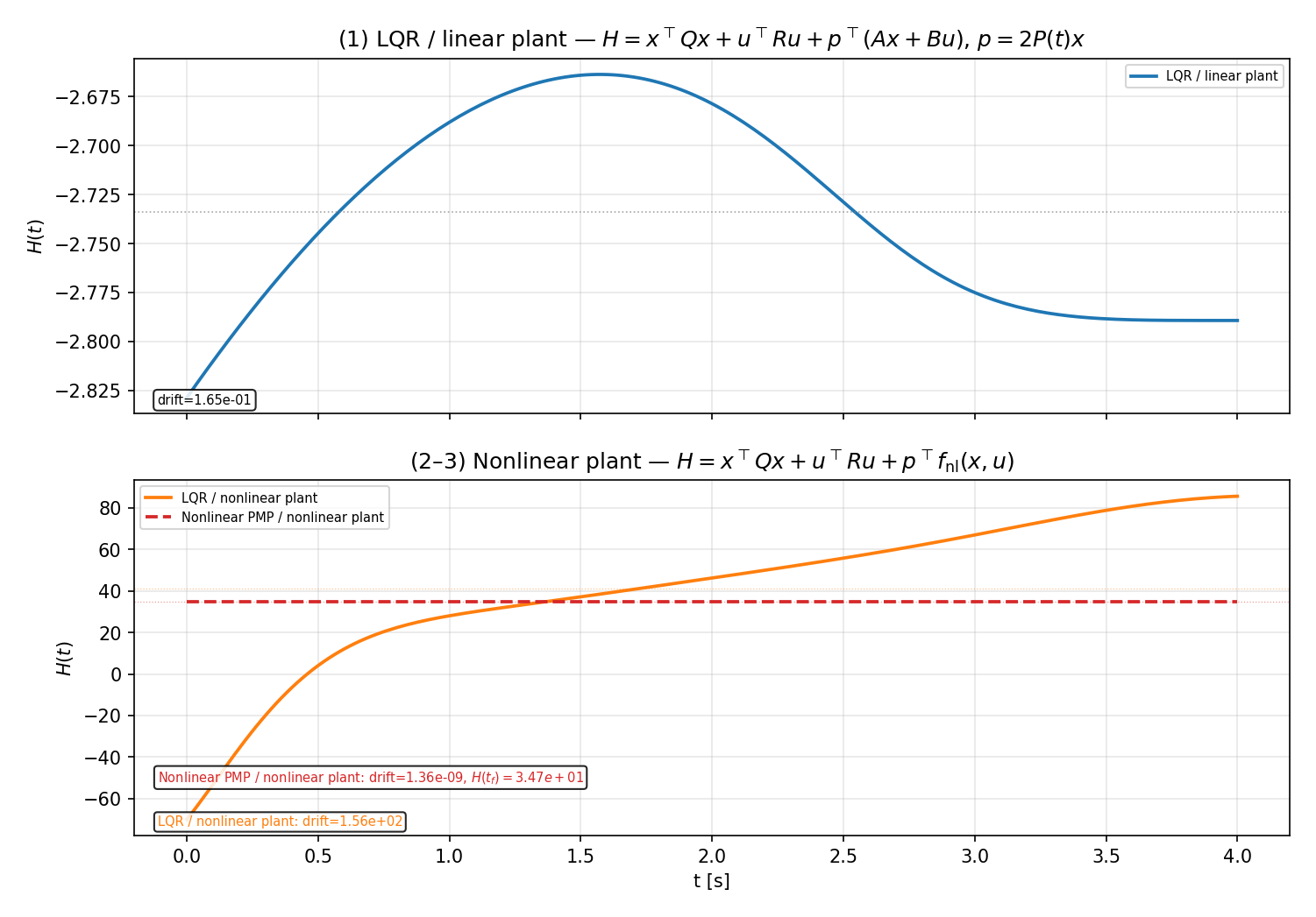
The nonlinear PMP solution holds $H$ constant to a drift of $O(10^{-9})$ about $H(t_f) \approx 34.7$. By contrast, applying the linear LQR law to the nonlinear plant produces a Hamiltonian that drifts by $O(10^2)$ over the same horizon — a direct, quantitative certificate that the linear law is not an extremal of the nonlinear problem.
| Type | Condition | Residual |
|---|---|---|
| Initial | $x(0) = x_0$ ($L_\infty$) | 3.9 × 10⁻²⁶ |
| Transversality | $p_{p_z}(t_f) = 2Q_{f,22}\,p_z(t_f)$ | 1.8 × 10⁻¹⁵ |
| Transversality | $p_\theta(t_f) = 2Q_{f,55}\,\theta(t_f)$ | 8.9 × 10⁻¹⁶ |
| Transversality | $p_\omega(t_f) = 2Q_{f,66}\,\omega(t_f)$ | 5.6 × 10⁻¹⁷ |
| Transversality | $p(t_f) = 2Q_f x(t_f)$ ($L_\infty$) | 1.8 × 10⁻¹⁵ |
| Hamiltonian | $H(t)$ drift (autonomous, fixed $t_f$) | 1.4 × 10⁻⁹ |
| Collocation | Interior RMS defect (219 nodes) | 9.7 × 10⁻⁷ |
Both the global $L_\infty$ boundary residual of 1.8 × 10⁻¹⁵ and the maximum interior collocation residual of 9.7 × 10⁻⁷ on a converged 219-node mesh fall within solver tolerance, confirming that the computed solution satisfies the necessary optimality conditions to numerical precision.
References
Nathan Ge
Department of Mechanical and Aerospace Engineering
University of California, Los Angeles
Email: nzge@g.ucla.edu
Acknowledgment
The author thanks Professor Shahriar Talebi for guidance and instruction throughout the MAE 270C Optimal Control course. Their insights into optimal control theory formed the foundation of this project.
-
D. Liberzon, Calculus of Variations and Optimal Control Theory: A Concise Introduction. Princeton University Press, 2012. ↩
-
A. E. Bryson and Y.-C. Ho, Applied Optimal Control. Routledge, 2018. [Online]. Available: https://doi.org/10.1201/9781315137667 ↩
-
D. E. Kirk, Optimal Control Theory: An Introduction. Courier Corporation, 2004. ↩
-
B. Acikmese and S. R. Ploen, “Convex programming approach to powered descent guidance for Mars landing,” Journal of Guidance, Control, and Dynamics, vol. 30, no. 5, pp. 1353–1366, 2007. [Online]. Available: https://doi.org/10.2514/1.27553 ↩