E.D.I.S.O.N. - Electronic Device for Installing Screws On (bulb) Nuts
I. Introduction
The guidelines for this project were to design, simulate, and construct a robotic manipulator arm with at least four degrees of freedom to accomplish a specific task. With our project, we aimed to create a robot capable of installing a lightbulb into a threaded socket. To achieve this task, we designed E.D.I.S.O.N., or more specifically, the Electronic Device for Installing Screws On (bulb) Nuts.
E.D.I.S.O.N. is composed of a planar RRR manipulator atop a revolving base with an end effector specifically designed for grasping a lightbulb, transporting it, and screwing it into the socket. To accomplish the three key characteristics of a robot: Sense, Plan, and Act, we looked at different options:
- Sense: We aimed to implement an ultrasonic sensor and camera to detect the lightbulb and socket locations, with respect to the manipulator’s base.
- Plan: We used forward and inverse kinematics introduced in lecture to convert the design’s specifications into corresponding equations used to control the location of each link in 3D space, which allowed us to determine the reachable workspace of the end effector.
- Act: We used five servo motors to create the RRR manipulator arm and revolving base that effectively and efficiently completed the task.
In the following sections, we dive deeper into the details of each aspect and discuss how we modified our initial plan to fit real-world design, manufacturing, and time constraints.
II. Manipulator Configuration
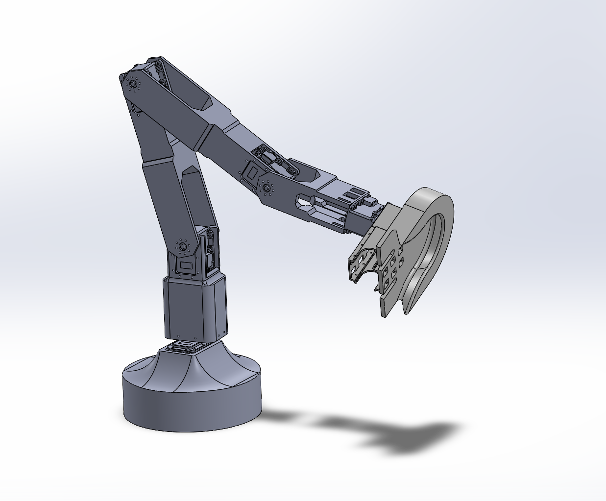
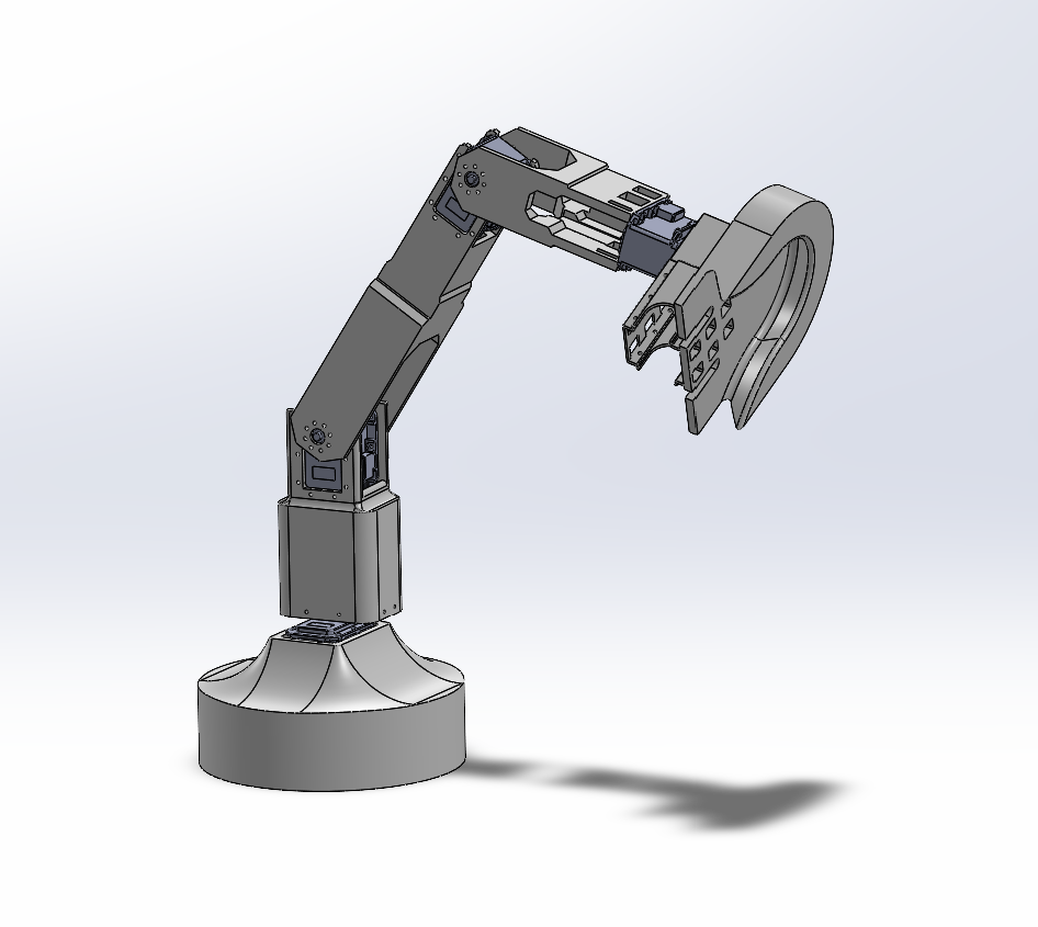
Our design of E.D.I.S.O.N., is a planar RRR manipulator on top of a revolving base. The links for each revolute joint are controlled by Dynamixel MX-28AR servo motors. The revolving base rotates solely around the world z-axis. This allows us to more easily rotate all links simultaneously, simplifying the kinematic calculations and greatly expanding the reachable workspace. Additionally, the end effector is attached to a continuous motor to achieve the screwing motion required to put in a lightbulb once the socket is reached.
Although different types of manipulators could have been used to achieve this task, the rotation motion used by humans to screw in a bulb proved to be the easiest method. Because the other links provided the degrees of freedom needed, the end effector’s revolute joint was enough to complete the task easily.
Our link design focused on structural strength, attempting to reduce the effects of shearing and bending induced by the large moments created by the servo motors. With the ultimate goal of reaching an overhead lightbulb socket in mind, we chose relatively long links. Our original, three-link design had a ground to end-effector reach of 75.53 cm, later shortened to 54.84 cm in our two-link design. These choices gave our robot excellent articulation and workspace range at the cost of having fairly heavy links and large torques acting on the motors, which, when paired with the heavy servos, led to future challenges.
III. Design Highlights and Difficulties
End Effector
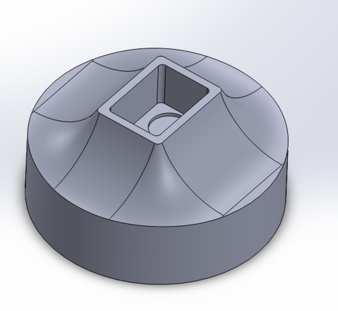
The end effector was designed to easily—yet securely—grasp and release the light bulb with sufficient room for error. Due to the vibrations generated when moving the manipulator arm, the walls of the end effector that come into contact with the bulb are splayed outwards to be as forgiving as possible upon entry. Once the bulb slides in, it is then grasped by a motorized attachment designed to apply downward force—as seen in Figure 3.2—increasing the force of friction between the end effector’s platform and the lightbulb’s face.
To screw the lightbulb in, the effector is mounted to the servo’s attachment. The effector’s axis of rotation is intentionally collinear with the symmetry axis of the lightbulb to minimize any forms of runout.
Base and Link 1
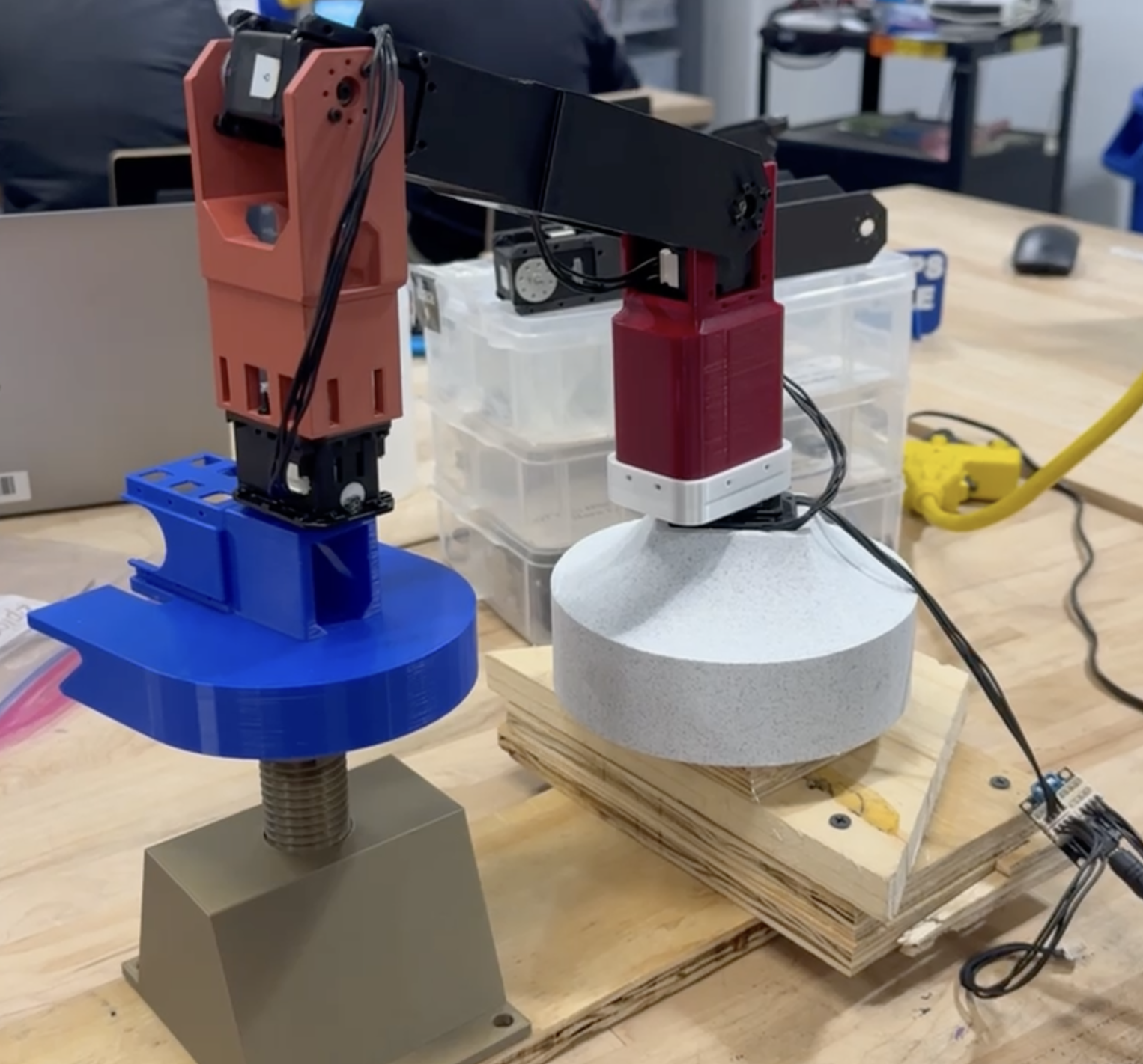
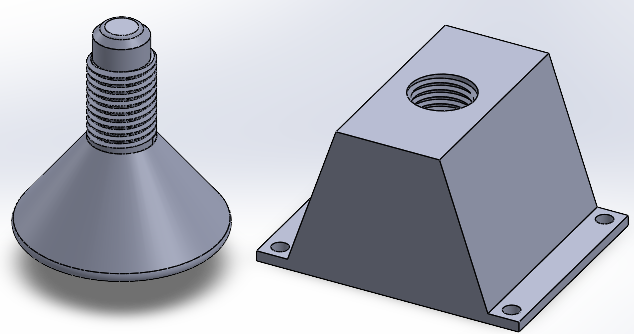
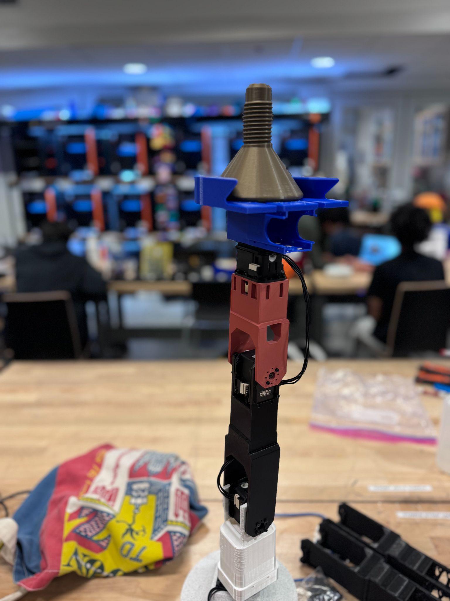
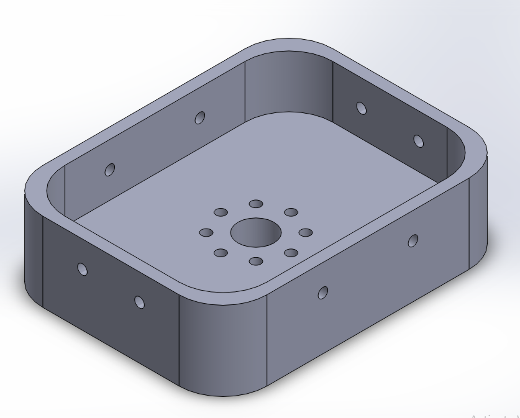
As seen in Figure 3.4, the base housed the motor for the rotation of the arm. This proved to be a suitable design for our motor configuration; however, it did not have the weight to support the whole arm. We had to attach the base to wood boards to ensure there was enough weight for the arm, as seen in Figure 2.2.
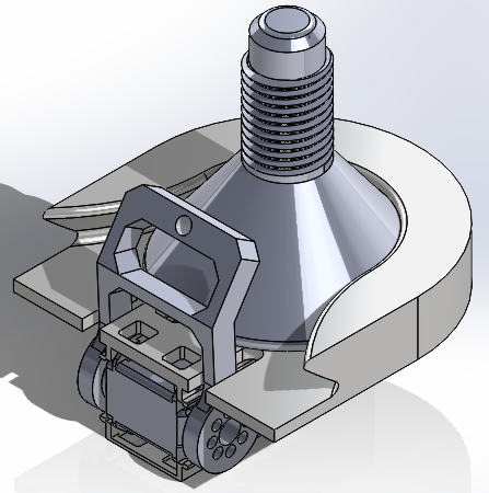
When designing the connector between the base and link 1, we observed that with the design of link 1, we would not be able to screw in the screws for the motor and attachment. Therefore, a secondary piece had to be designed to fit onto link 1 and was separate so that we could screw in the screws. As seen in Figure 3.6, this would have the proper screw holes and extrusions for link 1 to be placed inside. The other end of link 1 is equipped with prongs to act as mounts for the second motor, which would attach to link 2.
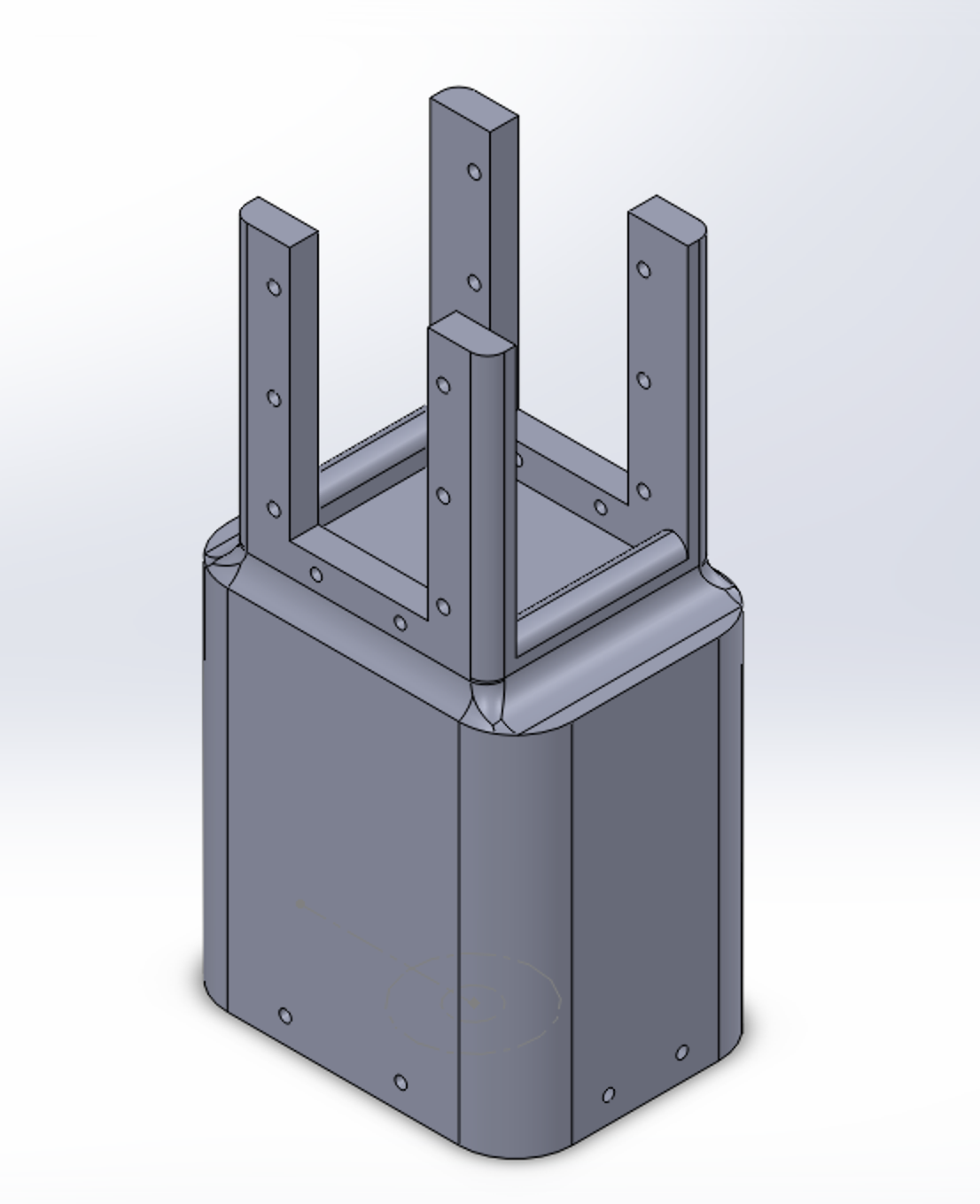
This design worked very well and helped secure a solid foundation for the rest of the links and the end effector. Additionally, circular cavities at the bottom link 1 helped ensure the screwheads from motor 1 did not prohibit a good fit for the holder and link 1.
IV. Derivation of Kinematics
Denavit-Hartenberg Parameters
| Joint | $\alpha_i$ | $a_i$ | $d_i$ | $\theta_i$ |
|---|---|---|---|---|
| 1 | $\pi/2$ | 0 | 0.123 m | $\theta_1$ |
| 2 | 0 | 0.186 m | 0 | $\theta_2$ |
| 3 | 0 | 0.186 m | 0 | $\theta_3$ |
| 4 | 0 | 0.196 m | 0 | $\theta_4$ |
Using the DH parameters from the table above describing the design of our system, the transformation matrix in Figure 4.1 was calculated using the provided Matlab code. The table above is organized in classic DH format as opposed to a modified format.
The transformation matrix from base to end effector frames is:
\[{}^{0}T_{4} = \begin{bmatrix} c_1 c_{234} & -c_1 s_{234} & s_1 & c_1(a_2 c_2 + a_3 c_{23} + a_4 c_{234}) \\ s_1 c_{234} & -s_1 s_{234} & -c_1 & s_1(a_2 c_2 + a_3 c_{23} + a_4 c_{234}) \\ s_{234} & c_{234} & 0 & d_1 + a_2 s_2 + a_3 s_{23} + a_4 s_{234} \\ 0 & 0 & 0 & 1 \end{bmatrix}\]where $c_i = \cos(\theta_i)$, $s_i = \sin(\theta_i)$, $c_{ij} = \cos(\theta_i + \theta_j)$, $s_{ij} = \sin(\theta_i + \theta_j)$, etc.
V. Solution Selection for Inverse Kinematics
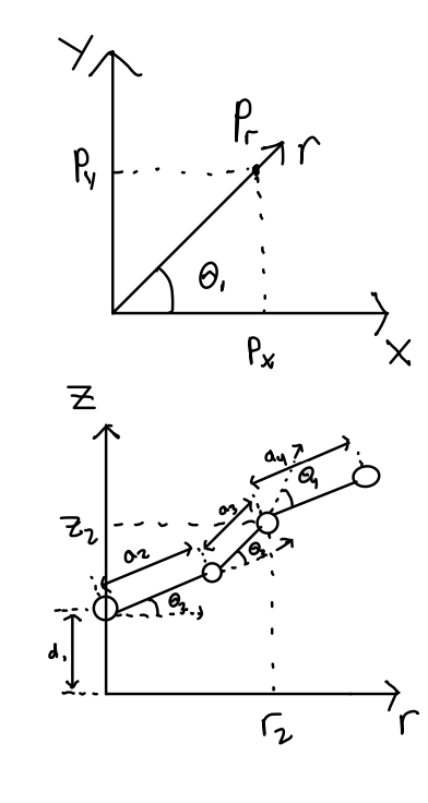
The inverse kinematics equations are derived from geometrical means from the diagrams of our system as well as using the transformation matrix in the forward kinematics:
\[\begin{aligned} \theta_1 &= \tan^{-1}\left(\frac{p_y}{p_x}\right) \\ p_r &= \sqrt{p_x^2 + p_y^2} \\ z_3 &= p_z - d_1 \\ \phi &= \theta_2 + \theta_3 + \theta_4 \\ r_2 &= r_3 - a_4 \cos \phi \\ z_2 &= z_3 - a_4 \sin \phi \\ \cos \theta_3 &= \frac{r_2^2 + z_2^2 - (a_2^2 + a_3^2)}{2 a_2 a_3} \\ \theta_3 &= \pm \cos^{-1}\left(\frac{r_2^2 + z_2^2 - (a_2^2 + a_3^2)}{2 a_2 a_3}\right) \\ \cos \theta_2 &= \frac{(a_2 + a_3 \cos \theta_3) r_2 + (a_3 \sin \theta_3) z_2}{r_2^2 + z_2^2} \\ \sin \theta_2 &= \frac{(a_2 + a_3 \cos \theta_3) z_2 + (a_3 \sin \theta_3) z_2}{r_2^2 + z_2^2} \\ \theta_2 &= \text{atan2}(\sin \theta_2, \cos \theta_2) \\ \theta_4 &= \phi - (\theta_2 + \theta_3) \end{aligned}\]For solution selection, it is important to prefer the elbow-up position for our robot manipulator so that it moves the links as high out of the way of obstacles when the whole system rotates about the z-axis from joint 1. Additionally, it is important that the end effector is facing towards the ground when it reaches its desired target position for our own use cases, as the lightbulb socket is oriented upwards.
VI. Workspace Analysis
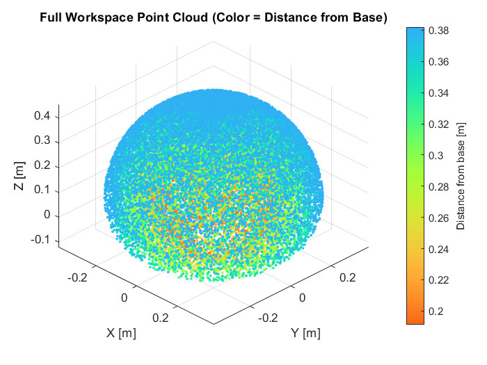
To determine the reachable workspace of the final robot design analytically, the forward and inverse kinematics were utilized to calculate which positions were located within and outside of the workspace. For the positions that could be reached, their locations in 3D space are plotted as a point cloud in Figure 6.1. To get a better understanding of the reachable workspace, a cross-section of the point cloud with a cutting plane in the x-z direction can be observed in Figure 6.2, which reveals a small void within the workspace. This void indicates further points that are not reachable by the current design, largely in part of the individual link lengths in the current design, in addition to the servo limits.
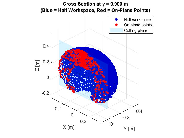
The current reachable workspace is very typical of most 3R robotic arms and did not produce any unexpected findings. It also allows for a variety of positions towards addressing the problem at hand, from loading a lightbulb at a particular point and then moving along a trajectory towards where the lightbulb needs to be screwed in. As long as the specified way points for each of these locations are within the point cloud, along with the trajectory between the two locations, there should be no issues for the robot to complete these tasks. Although this does not take into account dynamic limitations and changes as the robot moves throughout the reachable workspace, which may need further consideration if issues arise within the current reachable workspace.
VII. Task Simulation
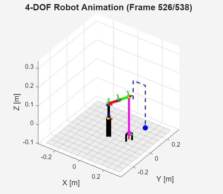
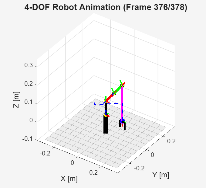
With the current design parameters, forward and inverse kinematics, and a target trajectory, we were able to simulate our robotic manipulator both from our initial design of a planar RRR and a planar RR manipulator, both atop a rotating base. Using the initial design, the first simulation for the robot was given a simple segmented trajectory to lift the end effector, move it across the x-y plane, and then descend the end effector in order to screw it into a target position.
In order to calculate these trajectories, each of the goal positions from the lightbulb load position to the lightbulb screw position can be represented as waypoints in 3D space 1. Additionally, desired points along the trajectory can be represented in the same fashion to ensure that the calculated trajectories lie within the reachable workspace outlined in Section VI. After defining the waypoints, parametric equations in the x, y, and z directions going through all of the waypoints are then calculated and finally simulated. This simulation demonstrates a possible routine our robot could follow in order to accomplish the task.
Figure 7.1 shows the results of the simulation, with each link colored uniquely and the intended trajectory displayed as a dashed line. When shifting to the final design, the previously calculated inverse kinematics were still utilized for the new simulations through locking the value of the joint, which was set to zero, and augmenting the link length of that specific joint accordingly. Figure 7.2 displays the results of the simulation from our final design.
VIII. Challenges and Future Improvements
Throughout the development process, a couple of challenges were encountered that required a change of approach.
Design Challenges
Our original design focused on emphasizing structural strength and workspace range at the cost of having long, heavy links. This weight created significant loads that could have potentially caused issues with the servos. As a result, we decided to remove our second link, shifting to an RRR design (instead of RRRR). This dramatically reduced the maximum load on our first loaded servo, both by having one less major link and servo to add weight, and by decreasing the length of the moment arm. However, we now had much less range of motion when it came to where our arm could reach, requiring us to use a set distance and height for the socket instead of our robot being able to reach anywhere within its workspace. This adjustment also caused challenges on the coding side, as our simulations and applications of kinematics now required the first two links to be in a line.
Development Process Challenges
We also encountered a variety of problems involving the parallel development of our hardware and code. Poor planning of our development and fabrication process left the part of our team responsible for coding with little to do until our physical design was finalized. Likewise, once the coding aspect became our main focus, the design portion of our team had little to do. Better planning of parallel development or assigning dynamic roles to our team members could have potentially prevented some of these problems and allowed us to work more efficiently. Additionally, as we iterated through different designs, changing the length of and number of our links, we encountered problems trying to adjust our code to the different specifications. If we redid this project, we likely would take on a more defined structure of prototype development or focus on the robustness of our code to better handle foreseeable changes.
Manufacturing Challenges
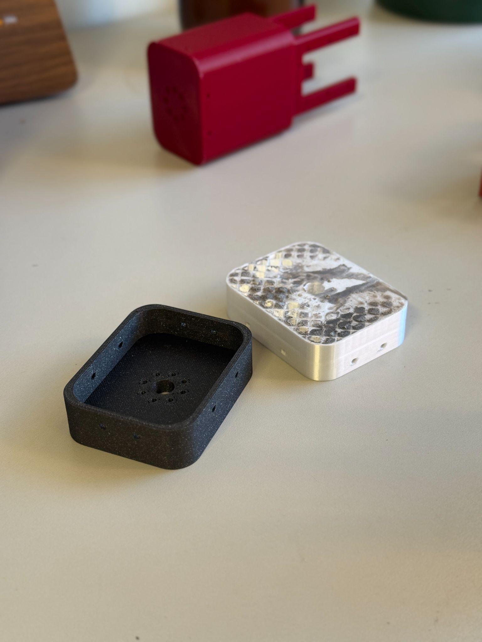
Furthermore, challenges with simple design aspects pushed back our timeline. Many issues stemmed from underestimating the screw sizes that were provided in the kit. The screwholes we intended to connect components were precisely 2mm (the thickness of the screws). We did not take into account the tolerance of the 3D printer and material, so many of the screws would not fit in the screwholes. As seen in Figure 8.2, our first iteration of the link 1 holder was too thick for the screw to pass through and connect to the motor (white component on the right). We had to sand down the piece, which ruined the structural integrity of the piece. Our second iteration (black component on the left) had a thinner profile and bigger screw holes to accommodate the tolerances in the real world.
Future Improvements
One of our primary future improvements would be to weight and moment-optimize an RRRR robot, allowing it to have the full, desired operating range of motion. In addition to cutting material and shortening links, coding the position to have the first link act as a counterweight could potentially help solve this problem. Adding a transmission to our second motor, programming a hard torque limit, or gain-scheduling a damper could also alleviate weight concerns if we reach the limit of our weight optimization.
Another improvement could be to build an overhead structure to hold the lightbulb socket in a more realistic position. Our end effector could also implement a sort of grasping mechanism, which would allow the arm to reach into an actual countersunk lightbulb socket instead of our idealized one and potentially become compatible with other sizes and shapes of bulbs. Adding a sensing element to find the hole, either with an ultrasonic sensor or a computer vision setup, is another improvement we would hope to make.
References
Ajay Chandrasekhar, Calvin Wicks, Cruz Ramirez, James Weiler, Liam McGlynn, Nathan Ge, Shahab Besharatlou
MAE C263A Final Project
Fall 2025