Characterization and Simulation of a Worm-Inspired Robot

Abstract

Soft-bodied invertebrates such as earthworms achieve efficient movement through coordinated peristaltic contractions of their body segments. This project explores this unique locomotive paradigm and examines its potential as a robotic framework.

I. Problem Statement

Traditional rigid robots struggle in confined spaces or irregular terrain (e.g., pipelines, soil, rubble). Soft-bodied worms offer a biological blueprint for adaptable motion via peristalsis. Understanding and simulating this mode of movement can inform the design of soft robots capable of traversing restrictive environments (e.g., medical endoscopy, search-and-rescue, pipeline inspection). Although peristaltic motion is effectively one-dimensional, it exhibits remarkable movement economy compared to limb-based locomotion, making it an efficient and robust strategy for soft robotic applications. The movement pattern is predictable yet surprisingly well-adapted to varied surface conditions, permitted surface contact can be maintained.

We gain insight into this mode of movement through the development of a computational model and simulation of a soft robotic worm. By capturing the coupling between actuation patterns, soft body mechanics and deformation, and frictional interactions with the environment, this model will provide insights into the fundamental physics and control strategies that enable efficient soft-bodied motion.

II. Background

Peristalsis Mechanics

It is first important to understand the underlying biomechanics that allow worms to move forward. The theory of peristalsis can then be shaped into a functional robot model.

At a high level, peristalsis is perceived as a wave-like propagation of muscle contraction and subsequent relaxation that is practiced repeatedly starting from the head to the toe of a worm’s body ¹². One contentious topic of discussion regarding the theory of peristalsis is the role of friction. Some believe friction is not the predominant source of movement, and that momentum transfer inside the body may be the driving mechanism. However, one way friction is believed to propel the worm is by providing a stationary anchor for segments in front of the actuated tissue to lurch forward ³. Simulation may reveal deeper truths about the mechanics of peristalsis.

However we may believe peristalsis drives forward locomotion, sequential wave-like contraction is the fundamental action that characterizes peristalsis, and any virtual or physical system should be built around this behavior.

Understanding the contraction pattern also means understanding the structure and supporting contractile elements that support this motion. The general structure of soft-bodied invertebrates is described as a hydrostatic skeleton, a type of skeleton supported by hydrostatic fluid pressure instead of rigid bony elements found in vertebrates. Worms retain their shape through the internal fluids that resist changes in volume. Forced changes in skeleton shape (contraction and relaxation) are governed by two major groupings of muscles. Longitudinal muscles that run along the length of the worm contract and extend axially, while circular, radial, and transverse musculature contract and extend radially. The paired action of these groups coordinated in a phase-based manner running along segments of the worm is what ultimately produces forward motion. Robotic systems must mimic the radial and longitudinal contraction efforts to respectively anchor and extend forward.

With the mechanics and the physical biological system understood, we can look to shape the structural makeup, actuation method, and control methodology of the bio-mimetic robot. These design aspects are inherently interdependent, each informing and constraining the others in the overall system design.

Material Construction

The robot’s exterior, or skeleton, so to speak, needs to be of pliable but durable/robust construction to accommodate a mode of actuation while being deformable to respond to actuation stimulus. This compliance of the structure can be of a mechanical nature (e.g., braided mesh) or achieved materially (stretchable elastomer).

Actuation Framework

A class of material important to the field of soft robotics is smart materials. They often couple some form of external stimulus to mechanical response. The study of smart materials and their application has proven substantive in the creation of robotic worms. Smart materials seek to directly manipulate the surface manifold to produce contraction and relaxation, such that the structure itself becomes the method of action.

Smart Materials

• Shape Memory Alloys (SMAs) ⁴ is one prevalent example of a smart material. They can reset back to a predefined structure when met with ample heat. They have the highest work density compared to other smart materials, meaning a small amount of material can generate a lot of work. They are not fast, but can behave responsively at microscale (such as the case of Micro helix SMAs, which have strain ratios of up to 200% and can be actuated in under a second). One implementation of SMA actuation has SMAs structures wrapped around the robot and actuated by wiring that also constitutes the braided mesh, creating seamless integration of actuation and structural framework.

• Dielectric Elastomers (DEAs) are another smart material that have a use case in building robotic worms ⁵. DEAs consist of a passive elastomer sandwiched between 2 compliant electrodes. Applied voltage acts between the electrodes and inadvertently squeezes the elastomer film through electrostatic pressure, causing expansion of material. DEAs can be shaped around a tube-like structure and actuated to mimic the pulsating activation pattern required for peristalsis.

• Ionic polymer–metal composites (IPMCs) ⁶: like DEAs, IPMCs are electroactive polymers. However, actuation is based on the migration/displacement of ions within a hydrated polymer matrix when a voltage is applied, causing the material to bend (a bimorph motion). IPMCs are slower in actuation compared to DEAs, but require low driving voltages.

Figure 1: A singular worm segment that contracts via dielectric elastomer actuation integrated into the bottom of the worm segment

Fluid-Based Actuators

Fluid-based actuators result in high force, precise, and controllable action that changes the shape of the worm from within. This action may perhaps more naturally mirror the biological model of actuation. However, they present their own set of limitations.

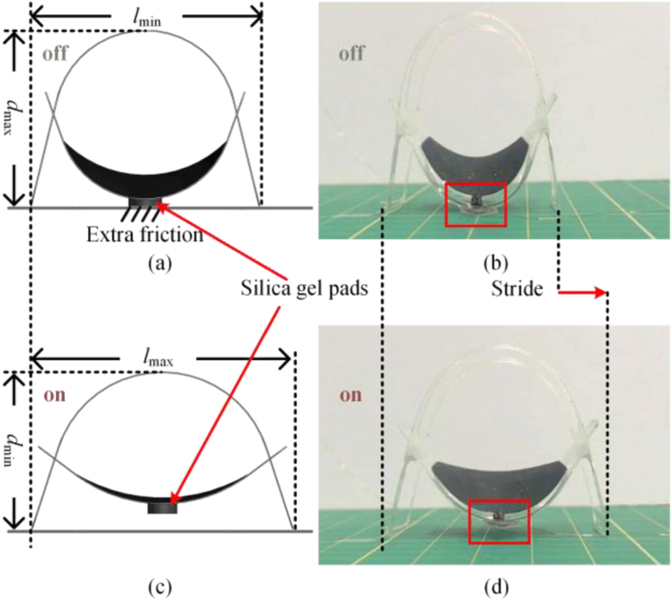
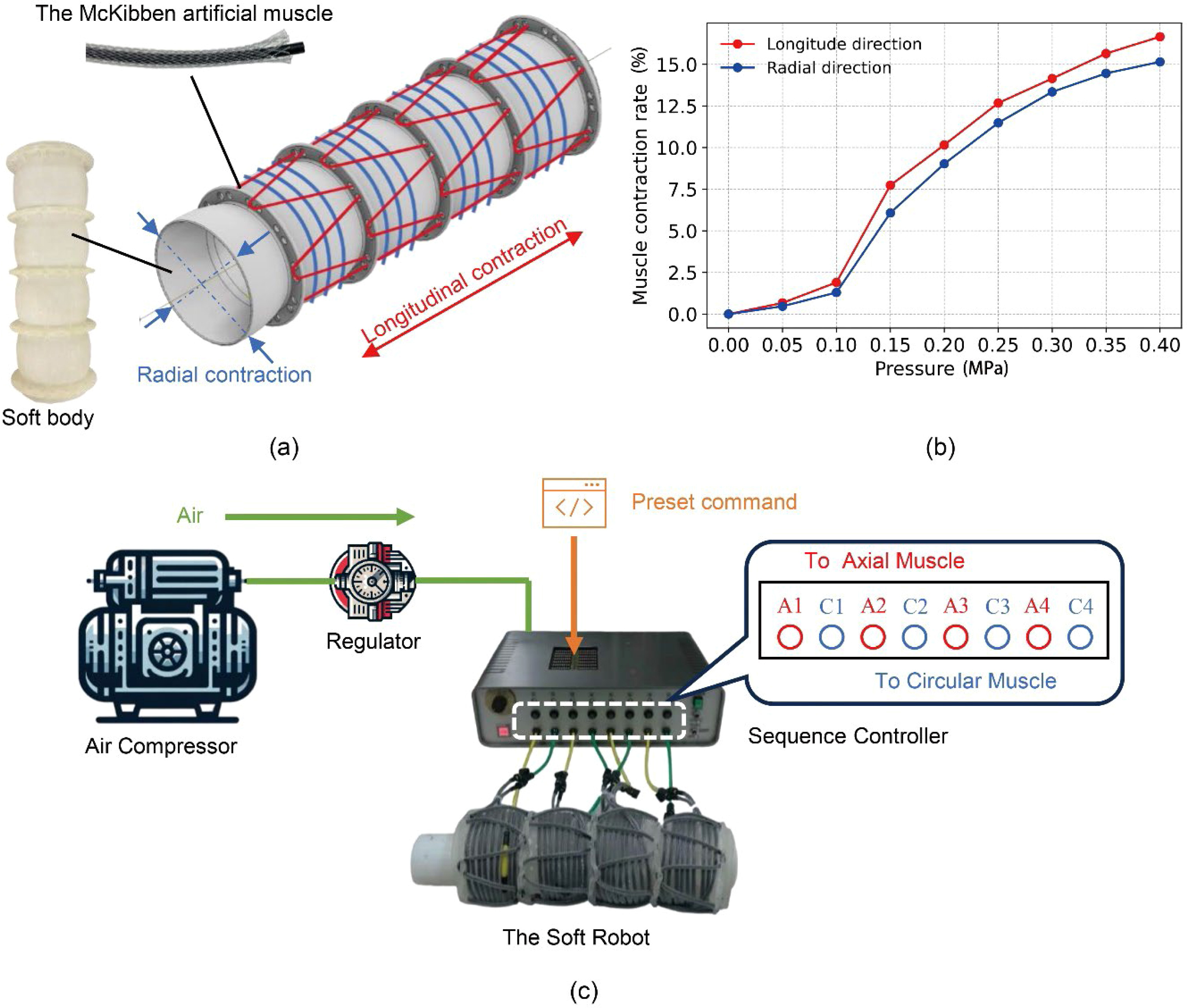
• Pneumatics ⁷: Movement of compressed air to drive contraction of artificial muscles contained with the skin wall. The theoretical basis of pneumatics is simple but hard to implement. Additionally, they require bulky pumps, resulting in an unwieldy construction.

• Hydrostatic Fluid Actuators: similar to pneumatics in that fluids are used to drive action. This method also has size scaling limitations, requiring an effective micro-hydraulic piston.

• Magnetic fluid ⁸: magnetic attraction of magnetic fluid embedded within the segmented worm as a permanent magnet passes over each self-contained body segment is one way to create patterned expansion. The challenge lies in the mechanism that moves the permanent magnet with minimal intervention.

Figure 2: Pneumatically actuated worm

Control Strategy

Depending on the locomotive intent of the worm robot, different control strategies can be employed to change the locomotive behavior of the robot.

Open Loop Control

The simplest control strategy employs an open-loop sinusoidal input applied to each body segment. This approach produces periodic contractions and relaxations that mimic biological peristalsis. When the actuation mode supports continuity, the control signal can be formulated as a continuous traveling sinusoidal wave along the worm’s body.

Intelligent Control Design

• Close loop: close-loop feedback control can be designed around certain measurable state variables, such as measure contraction/expansion of each segment (segment length/strain sensors) and position sensors (track head or body centroid movement). Local segment tracking combined with global body motion correction can be used to achieve a desired velocity.

• Stable heteroclinic channels (SHCs) ³: SHCs are a mathematical framework that allows smooth transitions between stable manifolds crossing unstable bridges.

• Neural Circuits ⁹: Neural circuit control design is inspired by biological neural drive operated through central pattern generators (CPGs). One study trained its neural CPG network on real Drosophila larvae by quantifying timing and duration of segmental boundary contractions. The network consists of repeated units of excitatory and inhibitory (EI) neuronal populations (for each worm segment) coupled with immediate neighboring segments. This model successfully generated forward and backward wave propagation.

Biomechanical Model

By building upon existing soft robotics modeling frameworks such as Cosserat rod formulations, this work aims to develop a computational foundation for studying efficient, biologically inspired soft locomotion. It is also important to match the computational framework to the intended mechanical system that achieves the bio-mimetic behavior. As we have discussed, the possible actuation methods and accompanying structures vary greatly even when applied to the same movement scheme.

But for the sake of capturing the worm’s end behavior to establish basic movement characteristics, most physical worm frameworks can be mathematically generalized to a simple 2-D planar model. The worm is first represented as a series of deformable planar (viewed from the side) segments actuated by a traveling contraction wave, enabling net forward motion through phase-shifted actuation.

Figure 3: 2D planar model using rhomboid linkages for height-length coupling

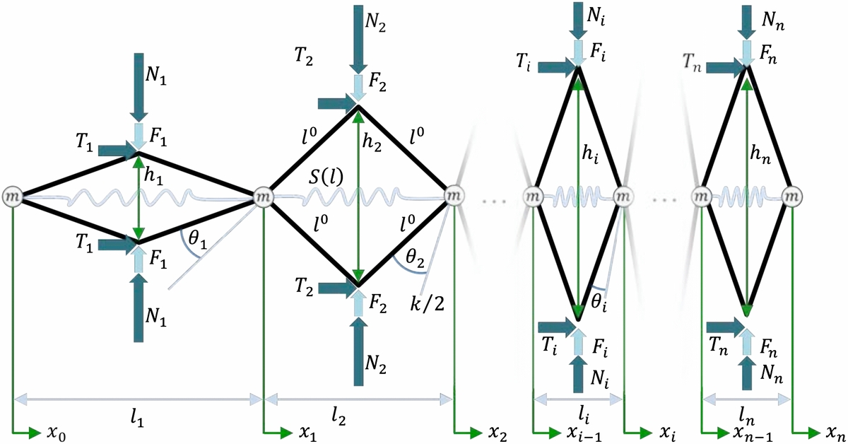
One model presents the worm as a segmented series of connected four-bar linkages that expand vertically and shorten horizontally when activated ³. This gives a more physically realistic coupling between radial and axial changes of each segment.

Figure 4: Turning worm model

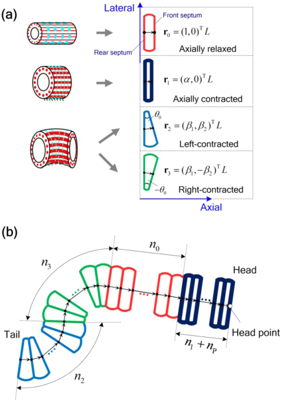
The model can then be further generalized to a 3-D structure ¹⁰. If rectilinear single-line motion is the goal, the 3-D generalization is more of a programming challenge of building surface geometry to better simulate frictional forces. However, the 3-D model also opens up the option of implementing turning capabilities. From a model perspective, the simplest implementation of turning is placing a rotational hinge in between rhomboid segments. Each time a segment is activated/contracted, a turning angle is applied to the hinge associated with the contracted segment. The approach that more realistically models a worm’s mode of turning action would be creating a differential radial actuation (left/right bias). Split the rhomboid into left and right chambers/tendons so you can inflate/contract them asymmetrically. If the left chamber expands more than right, the normal force distribution shifts and the body will bias to one side during sliding, which produces turning. The differential radial actuation may be a more physically realistic model and represents the neural intent of the worm, but the hinge integration is easier to build control frameworks around due to its relatively simpler dynamics.

Performance Metrics

The simulation will explore how actuation frequency, amplitude, and friction anisotropy influence locomotion performance. The results are expected to provide insight into control and design strategies for soft robots operating in constrained or complex environments. Segment count (representative of control fidelity, and perhaps the physical segment count of the final robot). Do more segments mean greater efficiency? The project will explore the relationship between actuation phase patterns and segment deformation, frictional interactions with the environment, and body compliance and stiffness distribution. An analytical framework surrounding these relationships and gain insight into locomotion efficiency and metabolic activity, maneuverability, stability, and control responsiveness to identify design parameters that optimize performance.

III. Simulation Approach

Model Construction

Figure 5: Rhombic linkage segments based worm model with 6 segments

Figure 6: Rhombic linkage segments based worm model construction description

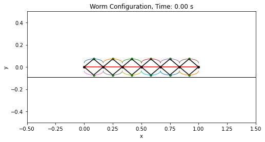
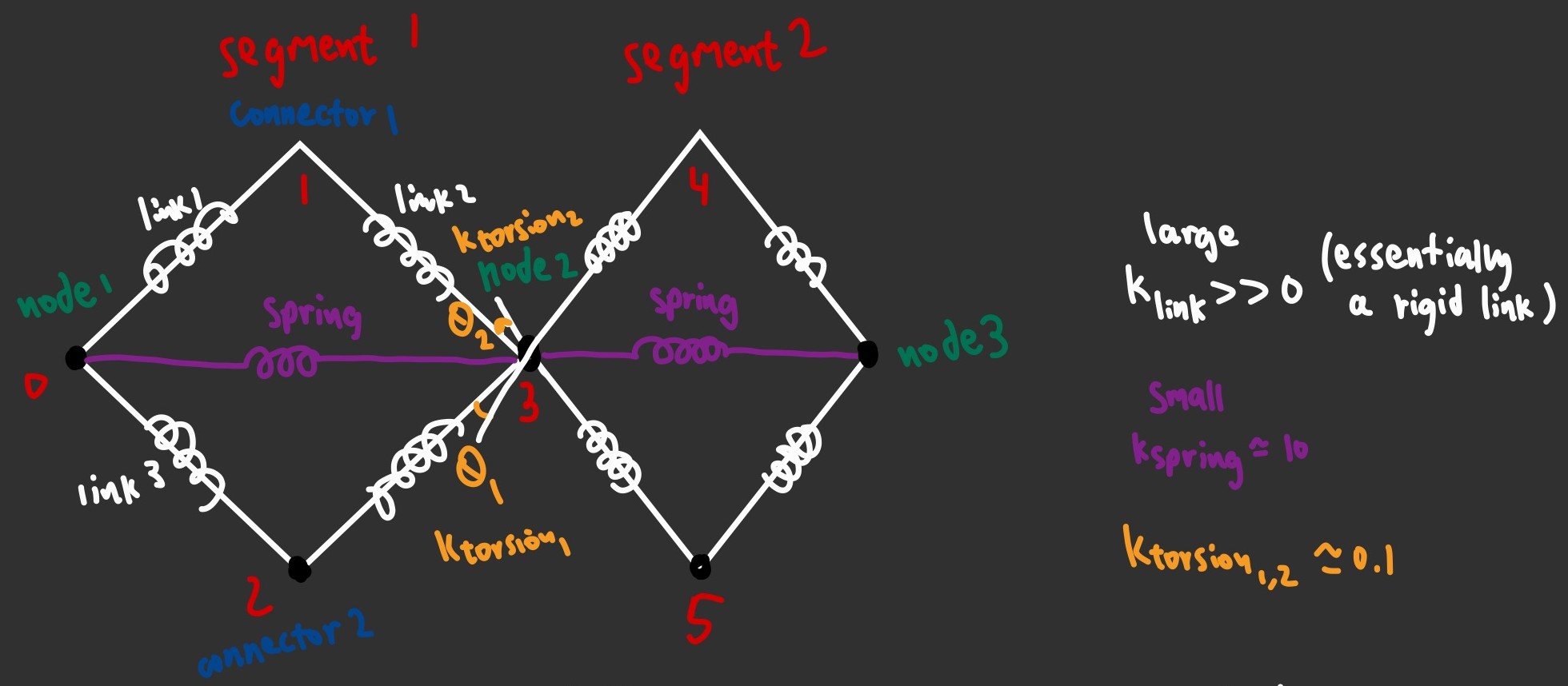
Each segment consists of a rhombic four-bar linkage. A linear spring extends horizontally across each segment to represent the natural elasticity of each segment. Torsional spring stiffness between segments represents a resistance to positional differences between adjacent segments.

Numerical Solver

Newton-Raphson Linearization and Implicit Eulers: Putting all contributions together, the Newton–Raphson equilibrium residual and Jacobian are:

\[\begin{aligned} \mathbf{f}(\mathbf{q}_{k+1}) &= \mathbf{F}_{\mathrm{inertia}} - \mathbf{F}_{\mathrm{elastic}} - \mathbf{F}_{\mathrm{viscous}} - \mathbf{F}_{\mathrm{friction}} - \mathbf{F}_{\mathrm{contract}},\\ \mathbf{J}(\mathbf{q}_{k+1}) &= \mathbf{J}_{\mathrm{inertia}} - \mathbf{J}_{\mathrm{elastic}} - \mathbf{J}_{\mathrm{viscous}}. \end{aligned}\]

At each time step we solve. We use the Implicit Euler method.

\[\Delta \mathbf{q} = -\mathbf{f}(\mathbf{q}_{k+1})/\mathbf{J}(\mathbf{q}_{k+1}), \qquad \mathbf{q}_{k+1} \leftarrow \mathbf{q}_{k+1} + \Delta \mathbf{q}.\]

The solver recomputes $f(q_{k+1})$ repeatedly until $f$ falls below a certain threshold that is approximately close to 0.

Predictor Corrector: A predictor–corrector scheme augments the Newton–Raphson solver by computing each Newton iteration potentially twice per solver iteration to correct for any errors given boundary conditions such as ground contact. In the predictor step, an explicit update (e.g., forward Euler) is used to generate a provisional estimate of the next state, $q_{k+1}^{0}$. This predicted value is then substituted into the system’s dynamics. In the corrector step, the method refines the solution by applying an implicit updated Newton iteration using the predicted state as the initial guess. The corrected value $q_{k+1}$ satisfies the force balance more accurately and typically reduces numerical drift and improves stability.

This predictor corrector setup is crucial for computing ground contact normal force for frictional force computations.

Force Balance: The quasi-static numerical solver minimizes the force of the following force balance equation at each time step.

\[\underbrace{\mathbf{M}\,\ddot{\mathbf{q}}}_{F_\text{inertia}} - \underbrace{\frac{\partial E^{\text{elastic}}}{\partial\mathbf{q}}}_{F_\text{elastic}} - \underbrace{\mu\mathbf{N}}_{F_\text{friction}} - \mathbf{F_{contract}} -\underbrace{\underbrace{\mathbf{C}\,\dot{\mathbf{q}}}_{F_\text{viscous}} - \underbrace{\mathbf{W}}_{F_\text{weight}}}_{\text{Optional}} = 0\]

Let \(\mathbf{q}_k\) and \(\mathbf{q}_{k+1}\) enote the generalized coordinates at times $t_k$ and $t_{k+1}$, and let \(\mathbf{u}_k\) denote the velocity at time $t_k$.

• The implicit Euler update gives the inertial contribution

\[\mathbf{F}_{\mathrm{inertia}} = \frac{m}{\Delta t} \left( \frac{\mathbf{q}_{k+1} - \mathbf{q}_k}{\Delta t} - \mathbf{u}_k \right), \quad \mathbf{J}_{\mathrm{inertia}} = \frac{\mathbf{M}}{(\Delta t)^2}.\]

• The spring linkage network contributes elastic stretching (from linear springs) and bending forces (from torsional springs)

  \[\begin{aligned} \mathbf{F}_{\mathrm{elastic}} &= \mathbf{F}_s(\mathbf{q}_{k+1}) + \mathbf{F}_b(\mathbf{q}_{k+1}), \\ \mathbf{J}_{\mathrm{elastic}} &= \mathbf{J}_s(\mathbf{q}_{k+1}) + \mathbf{J}_b(\mathbf{q}_{k+1}). \end{aligned}\]

  • The segment torsional spring energy model is as follows:

    \[\begin{aligned} E^{b} &= \frac{k_{\text{torsion}}}{2}\left(\Delta \text{cross}\right)^2 \\ \Delta \text{cross} &= \text{cross} - \text{cross}_0 \\ \text{cross} &= \mathbf{t}_1 \times \mathbf{t}_2 = t_{1x} t_{2y} - t_{1y} t_{2x} \\ \mathbf{t}_1 &= \frac{\mathbf{e}_1}{\lVert \mathbf{e}_1 \rVert}, \quad \mathbf{t}_2 = \frac{\mathbf{e}_2}{\lVert \mathbf{e}_2 \rVert} \\ \mathbf{e}_1 &= \mathbf{p}_b - \mathbf{p}_a, \quad \mathbf{e}_2 = \mathbf{p}_c - \mathbf{p}_b \end{aligned}\]

    The force (negative gradient) is:

    \[\mathbf{F}^t = -\frac{\partial E^t}{\partial \mathbf{q}} = -k_{\text{torsion}} \Delta \text{cross} \frac{\partial \text{cross}}{\partial \mathbf{q}}\]

    where $\mathbf{q} = [x_a, y_a, x_b, y_b, x_c, y_c]^T$ and:

    \[\begin{align} \frac{\partial \text{cross}}{\partial \mathbf{t}_1} &= [t_{2y}, -t_{2x}]^T \\ \frac{\partial \text{cross}}{\partial \mathbf{t}_2} &= [-t_{1y}, t_{1x}]^T \\ \frac{\partial \mathbf{t}_1}{\partial \mathbf{e}_1} &= \frac{\mathbf{I} - \mathbf{t}_1 \otimes \mathbf{t}_1}{l_1} \\ \frac{\partial \mathbf{t}_2}{\partial \mathbf{e}_2} &= \frac{\mathbf{I} - \mathbf{t}_2 \otimes \mathbf{t}_2}{l_2} \\ \frac{\partial \text{cross}}{\partial \mathbf{p}_a} &= -\frac{\partial \text{cross}}{\partial \mathbf{e}_1}, \quad \frac{\partial \text{cross}}{\partial \mathbf{p}_b} = \frac{\partial \text{cross}}{\partial \mathbf{e}_1} - \frac{\partial \text{cross}}{\partial \mathbf{e}_2}, \quad \frac{\partial \text{cross}}{\partial \mathbf{p}_c} = \frac{\partial \text{cross}}{\partial \mathbf{e}_2} \end{align}\]

    The Hessian (Jacobian) is:

    \[\mathbf{J}^t = -\frac{\partial^2 E^t}{\partial \mathbf{q}^2} = -k_{\text{torsion}} \left[ \frac{\partial \text{cross}}{\partial \mathbf{q}} \otimes \frac{\partial \text{cross}}{\partial \mathbf{q}} + \Delta \text{cross} \frac{\partial^2 \text{cross}}{\partial \mathbf{q}^2} \right]\]

    where the first term is the Gauss-Newton approximation and the second term includes second-order derivatives of the cross product with respect to positions.

  • The linear spring energy model is as follows:

    \[\begin{aligned} E^s &= \frac{k l_0}{2} \left(1 - \frac{l}{l_0}\right)^2, \\ \text{where } \quad l &= \sqrt{(x_{k+1} - x_k)^2 + (y_{k+1} - y_k)^2}. \end{aligned}\]

    The force (negative gradient) is:

    \[\mathbf{F}^s = -\frac{\partial E^s}{\partial \mathbf{q}} = \frac{k l_0}{2} \left(1 - \frac{l}{l_0}\right) \frac{1}{l l_0} \begin{bmatrix} -2(x_{k+1} - x_k) \\ -2(y_{k+1} - y_k) \\ 2(x_{k+1} - x_k) \\ 2(y_{k+1} - y_k) \end{bmatrix}\]

    where $\mathbf{q} = [x_k, y_k, x_{k+1}, y_{k+1}]^T$.

    The Hessian (Jacobian) is:

    \[\mathbf{J}^s = -\frac{\partial^2 E^s}{\partial \mathbf{q}^2} = \frac{k l_0}{2} \mathbf{H}^s\]

    where $\mathbf{H}^s$ is a $4 \times 4$ symmetric matrix with components:

    \[\begin{align} H^s_{ij} &= \frac{1}{l^2 l_0^2} \frac{\partial l}{\partial q_i} \frac{\partial l}{\partial q_j} + \left(1 - \frac{l}{l_0}\right) \left[ \frac{1}{l^3 l_0} \frac{\partial l}{\partial q_i} \frac{\partial l}{\partial q_j} - \frac{2}{l l_0} \delta_{ij} \right] \end{align}\]

    with $\frac{\partial l}{\partial \mathbf{q}} = \frac{1}{l} [-(x_{k+1} - x_k), -(y_{k+1} - y_k), (x_{k+1} - x_k), (y_{k+1} - y_k)]^T$.

• Viscous damping (if enabled) would produce the following. Although not important to the simulation, we could use this term to simulate worm locomotion through viscous media.

  \[\begin{aligned} \mathbf{F}_{\mathrm{viscous}} &= -\mathbf{C}\frac{\mathbf{q}_{k+1}-\mathbf{q}_k}{\Delta t}, \\ \mathbf{J}_{\mathrm{viscous}} &= -\frac{\mathbf{C}}{\Delta t}. \end{aligned}\]

  In the present model, $\mathbf{F}_{\mathrm{viscous}} = \mathbf{0}$.

• Ground contact is enforced using a predictor–corrector scheme in which normal forces are inferred from constraint residuals, and anisotropic Coulomb friction is applied based on the direction of tangential motion.

  \[N_i = \left| r_{y,i} \right| = \mathbf{F}_{\mathrm{ground}}(\mathbf{q}_k, \Delta t),\] \[F_{\text{friction},i} = \begin{cases} -\mu_{\text{forward}}\, N_i \, \mathrm{sign}(v_{x,i}), & v_{x,i} > \varepsilon, \\ -\mu_{\text{backward}}\, N_i \, \mathrm{sign}(v_{x,i}), & v_{x,i} < -\varepsilon, \\ 0, & |v_{x,i}| \le \varepsilon . \end{cases}\]

• Muscle activation / body contraction contributes the externally supplied force. The contraction pattern is discussed in detail in the control scheme portion.

  \[\begin{aligned} F_{\mathrm{contract}} &= \text{ContractionEngine}_{\text{segment-driven}} (\text{contractType}, T_{\mathrm{wave}}, T_{\mathrm{contract}}), \\ \text{OR} \\ F_{\mathrm{contract}} &= \text{StandingWaveContraction}(\phi(x,t)). \end{aligned}\]

Contraction

Two contraction strategies were explored. In both instances, the goal was to achieve a cyclical contraction sequences that enables forward propulsion.

Segment-by-segment contraction

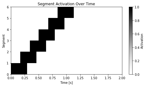
The ContractionEngine_segmentdriven class models a series of muscle-like segments that activate sequentially in a traveling wave pattern. Each segment has a contraction phase and generates a force pulse based on its phase. The engine operates in four steps:

1. Wave-Based Activation: Segments are activated in order along the body according to the current wave phase. Only one segment activates at a time per wave.

2. Phase Update: Active segments increment their contraction phase over time. Once a segment reaches its contraction duration ($T_{\text{contraction}}$), it deactivates and resets.

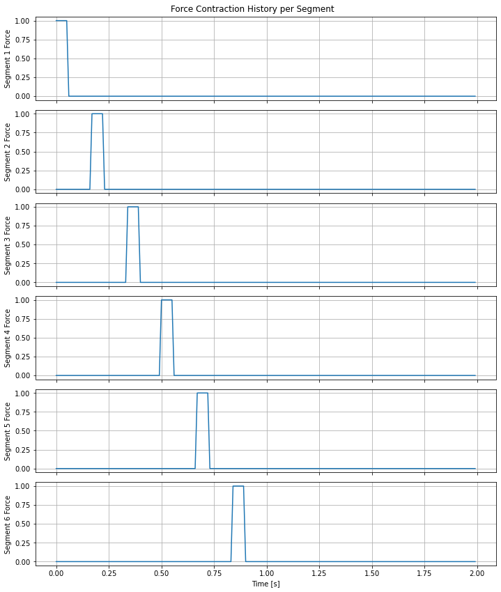
3. Pulse Generation: Each active segment produces a force according to a chosen pulse shape (gaussian, square, or dirac), based on its current contraction phase.

4. Force Computation: Segment forces are applied with alternating signs along the body to produce net directional force. Inactive segments contribute zero force.

This approach allows modeling of sequential, wave-like contractions and the resulting force distribution along a multi-segment body.

Figure 7: Segment based activation

Figure 8: Segment based contraction force

Standing/Traveling Wave Contraction Pattern

This contraction arguably models natural peristaltic contractions more accurately.

We prescribe a traveling-wave muscle activation pattern along the body:

\[x = \frac{i + \tfrac{1}{2}}{N}, \qquad x \in [0,1],\]

where $i$ indexes the segment and $N$ is the number of segments.

The temporal and spatial frequencies are

\[\omega = \frac{2\pi}{T_{\mathrm{wave}}}, \qquad k = \frac{2\pi}{\lambda}.\]

For a traveling wave from head ($x=0$) to tail ($x=1$), the activation phase is

\[\phi(x,t) = kx - \omega t,\]

and the contraction amplitude applied to each segment is

\[A(x,t) = \sin\!\left( \phi(x,t) \right) = \sin\!\left( kx - \omega t \right).\]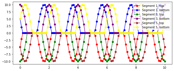

Figure 9: Standing wave contraction force

Control Framework

Velocity Based Control

Neural Intent

Stable Heteroclinic Channels

IV. Results

Locomotive performance is measured in Cost of Transport (COT). There are two ways to measure COT, one by measuring force application, another by measuring losses from friction.

The mechanical work done by actuation and the corresponding cost of transport contribution due to actuation over one time step is

\[W_{\text{contract}}^{(n)} = \mathbf{F}_{\text{contract}} \cdot \left( \mathbf{q}^{n+1} - \mathbf{q}^{n} \right).\] \[\text{CoT}_{\text{contract}}^{(n)} = \frac{ W_{\text{contract}}^{(n)}}{ \Delta x_{\text{COM}} }.\]

Similarly, the mechanical work dissipated by friction over one time and the the corresponding frictional cost of transport across one time step is

\[W_{\text{friction}}^{(n)} = \mathbf{F}_{\text{friction}} \cdot \left( \mathbf{q}^{n+1} - \mathbf{q}^{n} \right).\] \[\text{CoT}_{\text{friction}}^{(n)} = \frac{W_{\text{friction}}^{(n)}}{ \Delta x_{\text{COM}} }.\]

With the limited capabilities of the simulation to mirror true real world dynamics based on true physical parameters, benchmarks were run to gain a qualitative understanding of the relationship of segment count and contraction wave characteristics on Cost of Transport and locomotive speed. Here are all simulation parameters consistent across each simulation run:

Table I: Simulation Parameters for the Worm Model

Parameter	Value	Description
Model Parameters
$L$	$1.0~\mathrm{m}$	Worm length
$\rho$	$10~\mathrm{kg/m^3}$	material density
$k_\text{l-spring}$	$13$	[N/m] linear spring stiffness
$k_\text{link}$	$0.12$	torsional segment stiffness
$k_\text{torsion}$	$1e4$	[N-m/rad]torsional segment stiffness
Environment Parameters
$\mu_s$	$0.12$	Static friction coefficient
$\mu_k$	$0.10$	Kinetic friction coefficient
$\mu_{forward}$	$0.3\mu_k$	Forward friction coefficient
$\mu_{backward}$	$2\mu_k$	Backward friction coefficient
$\mathrm{tol}$	$EI/L^{2} \times 10^{-3}$	Solver tolerance
$\Delta t$	$0.01~\mathrm{s}$	Time step size
$T_{\text{total}}$	$10~\mathrm{s}$	Total simulation time
$N_{\max}$	$100$	Max Newton iterations

Workflow
The software pipeline is modular and experiment-friendly:

• Model Generation: Define worm length, number of segments, and fixed vertical DOFs.
• Solve: Run the implicit solver with contraction parameters and simulation time settings.
• Animate: Generate frame-by-frame renderings.
• Plot: Output center-of-mass progress, contraction energy, and cost-of-transport curves.

Segment Count test

I used the same contraction wave parameters on 5 different worms with different segment counts, ranging from 3 to 7 segments. The goal was to gain some qualitative insight into the effect of segment count on locomotive performance.

Table II: Simulation Parameters for Segment Count Test

Parameter	Value	Description
Model Parameters
$L$	$1.0~\mathrm{m}$	Worm length
$N$	$3,4,5,6,7$	Worm segment count
Contraction Wave Parameters
$\lambda$	$1.0~\mathrm{m}$	Contraction wave wavelength
$T_{wave}$	$2.0$	Wave Period

Figure 10: X-Direction Center of Mass tracked over 10 seconds from worms of different segment counts.

Figure 11: Cumulative Cost of Transport tracked over 10 seconds from worms of different segment counts.

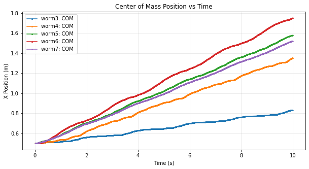
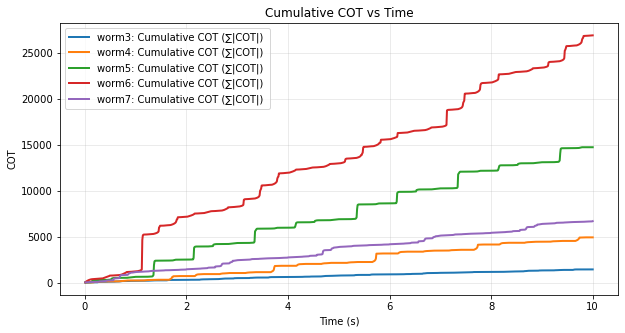
Distance traveled and cost of transport (CoT) generally increase as the number of segments increases. However, for the 7-segment worm, both metrics drop significantly compared to the 6-segment case.

Contraction profile analysis

I used the same six segment geometric worm model but altered the contraction wave parameters. Quantify the effect of wave period on propulsion.

Table III: Simulation Parameters for Contraction Profile Analysis

Parameter	Value	Description
Model Parameters
$L$	$1.0~\mathrm{m}$	Worm length
$n$	$6$	Number of segments
Contraction Wave Parameters
$\lambda$	$1.0~\mathrm{m}$	Contraction wave wavelength

Run A: $1.0~\mathrm{s}$ wave period
Run B: $2.0~\mathrm{s}$ wave period
Run C: $3.0~\mathrm{s}$ wave period
Run D: $4.0~\mathrm{s}$ wave period
Run E: $5.0~\mathrm{s}$ wave period

Figure 12: Center of mass tracked over 10 seconds from 6 segment worms of varying contraction wave periods.

Figure 13: Cumulative Cost of Transport tracked over 10 seconds from of varying contraction wave periods.

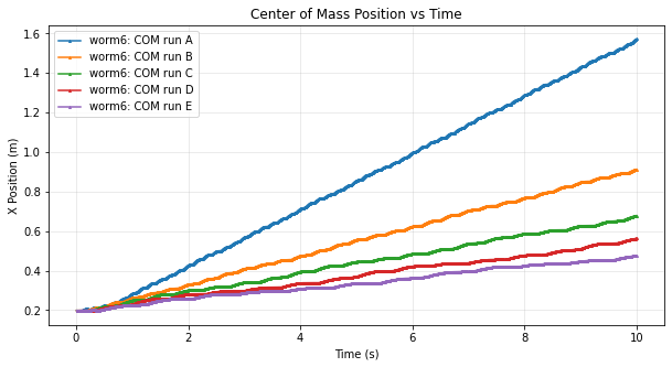
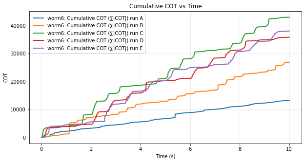
The results match intuition in that a shorter wave period produces more contraction efforts in a given time-frame, hence a higher Cost of Transport.

Current Challenges

The main challenges involve numerical stability:

• Mass distribution: Concentrating mass at nodes leads to unstable collapsed states.
• Torsional stiffness sensitivity: Extremely high torsion stiffness improves shape fidelity but destabilizes the Newton iterations.
• The y-axis of central nodes are clamped non-ideally to ensure numerical stability.

These instabilities restrict the parameter space over which the simulation can robustly produce physically realistic worm behavior.

V. Future Work

Solver: Future work will explore alternative numerical methods, such as a Hybrid pipeline that combines a fast real-time controller using Projective dynamics (PD)/Extended Peridynamic Model (XPDM), offline FEM-based validation, and a learned residual corrector. The residual corrector, implemented as a small neural network or regression model, would predict FEM-level residuals for unseen PD states, enabling real-time simulation with FEM-level accuracy. More realistic friction models will also be investigated, including enhanced predictor–corrector schemes and frictional anchoring forces in place of velocity-threshold-based formulations.

Contraction: Extensions to the current actuation model include non-rectified contraction profiles and alternative spatial–temporal contraction patterns to better replicate biological muscle activation.

Control Framework: Future control strategies include real time velocity regulation, Stable Heteroclinic Channels (often used in rhythmic pattern generation), and neural-intent-driven control (central pattern generators, CPGs, trained on real larval motion data could be used to generate biologically realistic contraction timing signals).

Environmental Factors: The model will be extended to more complex environments, including uneven or sloped terrain and confined pipe-like geometries that mimic real-life use cases.

Model Improvements: Additional work will focus on resolving numerical instabilities to enable more realistic simulations, incorporating spatially varying torsional and linear spring stiffnesses, and enabling path-following through directed contraction patterns using the modeling approaches discussed in the background.

VI. Conclusions

This project establishes a computational foundation for investigating efficient soft robotic locomotion. The insights gained from modeling actuation and body-environment interactions will guide the design of soft robots capable of adaptive and robust movement in complex settings.

References

---

Report

Nathan Ge
Department of Mechanical and Aerospace Engineering
University of California, Los Angeles
Email: nzge@g.ucla.edu

Acknowledgment
The author thanks Professor Khalid Jawed for guidance and instruction throughout the MAE 263F Soft Robotics course. Their insights into soft robotic modeling formed the foundation of this project.

^{4 1 2 5 3 11 12 10 13 8 14 9 6 15 7}

1. T. D. Nguyen, S. Park, and M. Sitti, “A new theory and methods for creating peristaltic motion in a robotic platform,” in Proc. IEEE Int. Conf. on Robotics and Automation (ICRA), 2010, pp. 1151–1156. [Online]. Available: https://ieeexplore.ieee.org/document/5509655 ↩ ↩²

2. Y. Uno, T. Ishihara, and M. Tanaka, “Locomotion strategy for a peristaltic crawling robot in a 2-dimensional space,” in Proc. IEEE/RSJ Int. Conf. on Intelligent Robots and Systems (IROS), 2007, pp. 2995–3000. [Online]. Available: https://ieeexplore.ieee.org/document/4543215 ↩ ↩²

3. R. Pfeifer, F. Iida, and G. Gómez, “Efficient worm-like locomotion: slip and control of soft-bodied peristaltic robots,” Bioinspiration & Biomimetics, vol. 8, no. 3, 2013. [Online]. Available: https://iopscience.iop.org/article/10.1088/1748-3182/8/3/035003 ↩ ↩² ↩³ ↩⁴

4. S. Coyle, E. Rouse, and C. Majidi, “Actuation and design innovations in earthworm-inspired soft robots: A review,” Frontiers in Robotics and AI, vol. 10, 2023. [Online]. Available: https://pmc.ncbi.nlm.nih.gov/articles/PMC9989016/ ↩ ↩²

5. H. Li, J. Zhang, and Y. Wang, “Development of an annelid-like peristaltic crawling soft robot using dielectric elastomer actuators,” Bioinspiration & Biomimetics, vol. 15, no. 4, 2020. [Online]. Available: https://iopscience.iop.org/article/10.1088/1748-3190/ab8af6 ↩ ↩²

6. M. Aureli, A. Pagano, and M. Porfiri, “Design and control of an IPMC wormlike robot,” IEEE/ASME Transactions on Mechatronics, vol. 15, no. 5, pp. 603–614, 2010. [Online]. Available: https://ieeexplore.ieee.org/document/1703647 ↩ ↩²

7. “Soft Pneumatic Earthworm Robots,” Arm Lab, Georgia Institute of Technology. [Online]. Available: https://armlab.gatech.edu/research-2/current/soft-pneumatic-earthworm-robots/ ↩ ↩²

8. T. Kato, K. Shimizu, and M. Sato, “Development of a peristaltic crawling robot using magnetic fluid on the basis of the locomotion mechanism of the earthworm,” Smart Materials and Structures, vol. 13, no. 3, pp. 362–368, 2004. [Online]. Available: https://iopscience.iop.org/article/10.1088/0964-1726/13/3/016/pdf ↩ ↩²

9. B. Gjorgjieva, J. Berni, and A. H. Cohen, “Neural circuits for peristaltic wave propagation in crawling Drosophila larvae: analysis and modeling,” Frontiers in Computational Neuroscience, vol. 7, 2013. [Online]. Available: https://www.frontiersin.org/articles/10.3389/fncom.2013.00024/full ↩ ↩²

10. Y. Luo, W. Zhao, and H. Yang, “In-plane gait planning for earthworm-like metameric robots using genetic algorithm,” Bioinspiration & Biomimetics, vol. 15, 2020. [Online]. Available: https://iopscience.iop.org/article/10.1088/1748-3190/ab97fb ↩ ↩²

11. H. N. Luu and S. Kim, “Controlling a peristaltic robot inspired by inchworms,” Artificial Life and Robotics, vol. 29, 2024. [Online]. Available: https://www.sciencedirect.com/science/article/pii/S2667379724000044 ↩

12. K. Takahashi and H. Kimura, “Peristaltic crawling robot based on the locomotion mechanism of earthworms,” in Proc. Int. Symp. on Micro-NanoMechatronics and Human Science, 2005, pp. 115–120. [Online]. Available: https://www.sciencedirect.com/science/article/pii/S1474667015341550 ↩

13. K. Yasuda, A. Nabae, and T. Morita, “Acquisition of earthworm-like movement patterns of many-segmented peristaltic crawling robots,” Journal of Intelligent Material Systems and Structures, vol. 27, no. 15, pp. 2045–2056, 2016. [Online]. Available: https://journals.sagepub.com/doi/10.1177/1729881416657740 ↩

14. C. T. Nguyen and M. Sitti, “A worm-like biomimetic crawling robot based on cylindrical dielectric elastomer actuators,” Frontiers in Robotics and AI, vol. 7, 2020. [Online]. Available: https://www.frontiersin.org/articles/10.3389/frobt.2020.00009/full ↩

15. Z. Xu, J. Zhang, and T. Li, “An earthworm-like modular soft robot for locomotion in multi-terrain environments,” Scientific Reports, vol. 13, 2023. [Online]. Available: https://www.nature.com/articles/s41598-023-28873-w ↩